6 Case Study: More Results from Note Taking Studies
In this chapter we will apply what we have learned in the previous chapter - how to analyse experimental data with one experimental manipulation and two conditions. For this, we will again take a look at the data from Urry et al. (2021). Additionally, we will analyse data from Mueller and Oppenheimer (2014). This study was the first published study investigating the question of note taking with a laptop or in longhand format and was the basis on which Urry et al. (2021) planned their study. For the data of Mueller and Oppenheimer (2014) we will perform a full analysis starting with reading in the data. So in addition to performing the statistical hypothesis test, we will calculate some descriptive statistics.
We start the analysis in this chapter in the same way as in the previous chapter, by loading the three packages we generally use, afex, emmeans, and tidyverse, and set a nicer ggplot2 theme. Before doing so it is probably a good idea to restart R (unless, of course, you are just starting R). In RStudio this can be conveniently done through the menu by clicking on Session and then Restart R. In other R environments you might need to restart the program. The benefit of restarting R is that it should create a blank R session in which no packages are loaded and no objects exist in the workspace. Only such a blank sessions ensures that, once we have obtained a set of results, we can recreate them later using the same code. That is, a blank R session avoids any potential problems due to analyses performed in a previous session that are still lingering. Restarting R should generally be done when starting a new analysis or after one is completely done with an analysis. In the latter case, it makes sense to restart R and the rerun all code one has saved in ones script to ensure that all results replicate based on only the code in the script (and do not require some additional code not saved).
library("afex")
library("emmeans")
library("tidyverse")
theme_set(theme_bw(base_size = 15) +
            theme(legend.position="bottom",
                  panel.grid.major.x = element_blank()))
6.1 Conceptual Memory Data from Urry et al. (2021)
As a quick reminder, Urry et al. (2021) showed their participants short lectures (TED talks) on video during which participants were allowed to take notes. One group of participants, the laptop condition, could take notes on a laptop, whereas the participants in the longhand condition could take notes with pen and paper. After the lecture, participants were quizzed on two aspects of the content of the lecture, factual questions and conceptual questions.
For example one of the videos is by Kevin Slavin on "How Algorithms Shape Our World". A factual question for this video was: "In New York City, where is the Internet distributed from?" A conceptual question for this video was: "How are algorithms useful for successful stock trading?"
In the previous chapter (5), we have analysed the overall memory score. The overall memory score was the average of the memory scores for the factual questions and the conceptual questions. In the present analysis, we are only concerned with the memory performance for conceptual questions.
We begin the analysis by reading-in the data. As it is part of afex, it can be read-in by calling the data() command (this only works after afex is attached with library()). We then get an overview of the variables using str().
data("laptop_urry")
str(laptop_urry)
#> 'data.frame':    142 obs. of  6 variables:
#>  $ pid       : Factor w/ 142 levels "1","2","4","5",..: 1 2 3 4 5 6 7 8 9 10 ...
#>  $ condition : Factor w/ 2 levels "laptop","longhand": 1 2 2 1 2 2 1 2 2 1 ...
#>  $ talk      : Factor w/ 5 levels "algorithms","ideas",..: 4 4 2 5 1 3 5 2 5 4 ...
#>  $ overall   : num  65.8 75.8 50 89 75.6 ...
#>  $ factual   : num  61.7 68.3 33.3 85.7 69.2 ...
#>  $ conceptual: num  70 83.3 66.7 92.3 82.1 ...
As before, we have the participants identifier variable in pid and the note taking condition in variable condition. We can also guess that the conceptual memory scores are in the aptly name variable conceptual (if we were unsure about this, we could also check the documentation of the data at ?laptop_urry).
Usually, once the data is sufficiently prepared (i.e., we have performed some coherence checks and identified DV and IV), the first step in an analysis should be plotting the data. This could be done using ggplot2 directly. However, in the present case it is very clear which statistical model we are going to estimate. In such a case, using afex_plot() involves a bit less typing. Thus, we start by estimating the statistical model for the conceptual memory performance of the data from Urry et al. (2021) and save the estimated model object as mc_urry (mc = model conceptual scores) . For this, we again use aov_car() on the laptopt_urry data and specify the statistical model using the formula interface. The DV we are considering here is conceptual, our IV is condition, and the participant identifier is pid. Consequently, the formula is conceptual ~ condition + Error(pid). Then, before looking at the inferential statistical results, we use this model object to plot the data using afex_plot.
mc_urry <- aov_car(conceptual ~ condition + Error(pid), laptop_urry)
#> Contrasts set to contr.sum for the following variables: condition
afex_plot(mc_urry, "condition")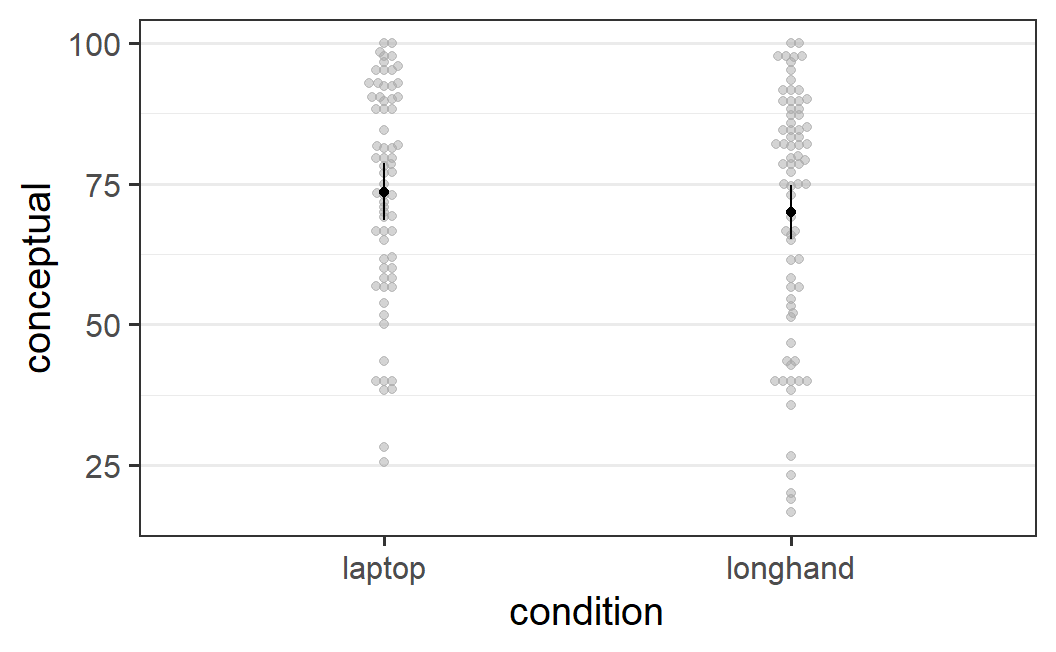
Figure 6.1: Conceptual memory scores from Urry et al. (2021) across note taking conditions
The reason for beginning with plotting the data is that it allows to see whether the data looks alright. That is, we check whether there are any features that stand out, such as single observations with extreme values ("outliers") or other unusual patterns. If this were the case, we would try to figure out if we can find a reason for the issues and how we want to deal with them. But, as the data looks alright, we continue and consider the results of the significance test:
mc_urry
#> Anova Table (Type 3 tests)
#>
#> Response: conceptual
#>      Effect     df    MSE    F  ges p.value
#> 1 condition 1, 140 441.76 1.00 .007    .319
#> ---
#> Signif. codes:
#> 0 '***' 0.001 '**' 0.01 '*' 0.05 '+' 0.1 ' ' 1
The ANOVA table reveals that the significance test for the effect of condition is not significant, with \(p = .319\). Thus, in line with the finding that there is no evidence for a difference in overall memory performance, there also is no evidence for a difference in memory for conceptual information.
We then also employ emmeans, for investigating the condition means (or estimated marginal means). In line with Figure 6.1, the memory score in the laptop condition is descriptively around 3.5 points higher than the score in the longhand condition. This is not too surprising, afex_plot uses emmeans internally. Therefore, the means shown in the figure above are exactly the same values as the means shown below.
emmeans(mc_urry, "condition")
#>  condition emmean   SE  df lower.CL upper.CL
#>  laptop      73.5 2.55 140     68.5     78.6
#>  longhand    70.0 2.44 140     65.2     74.8
#>
#> Confidence level used: 0.95
Before moving to the next data set, let's consider how we could report this analysis in a research report. For example, we could write:
As shown in Figure 6.1, participants' conceptual memory scores (on a scale from 0 to 100) are descriptively slightly larger in the laptop condition compared to the longhand condition. We analysed these scores with an ANOVA with one factor, note taking condition, with two levels (laptop vs. longhand). The effect of note taking condition was not significant, \(F(1, 140) = 1.00\), \(p = .319\). This indicates that the data does not provide evidence for a difference in memory for conceptual information based on how notes are taken during video lectures.
6.2 Why are Experiments Replicated?
The experiment by Urry et al. (2021) was not the first experiment investigating the effect of the type of note taking during lectures on memory. In contrast, their study was a replication of Mueller and Oppenheimer (2014). A replication is the act of repeating a previous study that has the goal of checking if one can obtain (or replicate) similar results as the previous study.
As we have discussed before, inferences from NHST are never conclusive as they are probabilistic and require multiple inferential steps. Replications are one of the most important tools in science for overcoming at least the probabilistic uncertainties associated with the inferences we draw from experimental data. For example consider that several independent but otherwise as similar as possible experiments – that is, replications of the same experiment – all obtain a significant result (i.e., indicate that the data are incompatible with the null hypothesis). Such a pattern would dramatically increase our confidence that the null hypothesis is likely false. In other words, replication studies are the main tool for overcoming the second inferential gap identified in Section 1.3.2.
In addition to the gain in confidence for specific results, there are good practical reasons for replicating an existing experiment. For example, when beginning to work on a new topic it is generally a good idea to replicate the experiment on which one wants to build on. If one already encounters problems replicating the results reported in the literature, this suggests that the topic may be less well-understood as portrayed in the literature.
Another excellent reason for performing a replication is not believing an existing result. Remember, one of the key components of the scientific method is scepticism (at least according to Wikipedia). And if a result is difficult to believe, the reasonable sceptical position is to require more evidence. A replication is one way – if not the best way – to produce additional evidence for a particular empirical finding. Not believing existing experiments also does not imply that one questions the integrity of the researchers who did the experiment. There are many completely harmless reasons why a study might not replicate. For example, researchers might have just obtained a significant results by chance (which happens in 5% of cases, as discussed in the next chapters).
Sadly, replicating existing experiments and publishing the results, is still not the norm in psychology and related disciplines. Quite to the contrary, the situation is so dire that many fields are currently considered to be in a replication crisis. For example, a large scale effort to replicate 100 studies in psychology (Open Science Collaboration 2015) showed that less than 50% of studies could be successfully replicated. Similarly sobering results have since been observed across the social sciences (Camerer et al. 2018, 2016; Klein et al. 2018). Much has been written about this problem and this is not the right place to rehash all arguments. The best summary of the situation is the book by Chris Chambers (Chambers 2017). The important thing is to realise that science is a cumulative endeavour. Every new experiment builds on existing research. If the existing research has never been replicated, our confidence in this research has to be low. This questions the foundations of any new work that builds on this non-replicated research. To move forward we researchers need to replicate work that is important for our research, value replications done by others (especially if it is of our own work), and let findings that do not replicate fade into obscurity.
6.3 Conceptual Memory Scores from Mueller and Oppenheimer (2014) Experiment 2
As Urry et al. (2021) is a direct replication of Mueller and Oppenheimer (2014), the design is the same and uses the same materials (i.e., the same TED talks and same questions). Participants watched short lecture videos (projected onto a screen) and could take notes either on a laptop or with longhand format. 30 minutes after the lecture they were asked factual and conceptual questions about the lectures. Their answers were coded by the first author. As in the previous analysis, we will transform the answers to a memory score from 0 (= no memory) to 100 (= perfect memory). In line with the analysis of Urry et al. (2021) above, we are only interested in the conceptual memory scores here.
The experiment by Urry et al. (2021) was a direct replication of Experiment 1 of Mueller and Oppenheimer (2014). Here, we first focus on Experiment 2 of Mueller and Oppenheimer (2014), which is also a direct replication of their Experiment 1 that only included an additional experimental manipulation which we will ignore. The reason for focussing on their Experiment 2 first is that the data is a bit more straightforward to interpret. We will get back to their Experiment 2 below, before providing a complete overview of the results of all data sets investigating the research question of whether the mode of taking note during lectures affects memory that employ the experimental design introduced by Mueller and Oppenheimer.
Luckily for us, the data from Mueller and Oppenheimer (2014), including the data from their Experiment 2, is available online on the Open Science Framework (OSF). The OSF is one of the most visible developments resulting from the replication crisis. It is a free website that allows researchers to share their data and other materials associated with their research. Before the replication crisis and the OSF, it was very rare to get access to the data underlying published studies. Nowadays, many researchers depose their (anonymised) data for published studies on the OSF and include the links to the data in their papers. This allows other researcher, such as us, to reanalyse existing data and ensure that the reported results can be reproduced.
Note that in this book we distinguish reproducing a result from replicating a result. Reproducing means being able to obtain the exact same results using the exact same data. That is, when given the data and the analysis script or a description of the analysis, we can perform the statistical analysis and end up with the same result. In contrast, replication means repeating the study with new participants and being able to obtain the qualitatively same result. In other words, replicating necessarily entails collecting new data whereas reproducing is based on the same data.
6.3.1 Preparing the Data
To get into the habit of downloading data from the OSF and reanalysing them, this is what we are going to do now. The file we need is called Study 2 abbreviated data.csv and can be found at the following OSF link: https://osf.io/t43ua/ Please go ahead and download it now and put it into your data folder so you can access it.
Because we use the original data available on the OSF, preparing the data for analysis involves more steps than our previous analyses. For example, we first need to figure out which variables and observations are relevant. We also perform a few simple coherence checks to make sure that our assumptions about the variables and data hold. Such a more involved data preparation phase, which also requires knowledge about the experiment, paints a more realistic picture of a data preparation. When doing so for ones own data, one also should spend some time on checking that there are no problems with the data.
The data preparation heavily draws on the tidyverse knowledge introduced in Chapter 3. We use function read_csv() to read-in the data and assign it to object mo2014_e2. As a reminder, read_csv() always returns a tibble (the tidyverse version of a data.frame). Then we use the glimpse() function (also a tiydverse function) to get an overview of the data (it is very similar to str() but less verbose for some tibbles).
mo2014_e2 <- read_csv("data/Study 2 abbreviated data.csv")
glimpse(mo2014_e2)
#> Rows: 153
#> Columns: 22
#> $ participantid            <dbl> 103, 122, 142, 152, 172, …
#> $ notetype                 <dbl> 1, 1, 1, 1, 1, 1, 1, 1, 1…
#> $ whichtalk                <dbl> 1, 1, 1, 1, 1, 1, 1, 1, 1…
#> $ Wcount                   <dbl> 148, 273, 124, 149, 182, …
#> $ threeG                   <dbl> 0.08219178, 0.05535055, 0…
#> $ factualindex             <dbl> 2.499, 2.833, 2.333, 4.49…
#> $ conceptualindex          <dbl> 2.0, 1.5, 2.0, 2.0, 2.0, …
#> $ factualraw               <dbl> 6, 7, 5, 11, 12, 4, 7, 11…
#> $ conceptualraw            <dbl> 4, 3, 4, 4, 4, 3, 4, 3, 4…
#> $ perfectfactindexscore    <dbl> 7, 7, 7, 7, 7, 7, 7, 7, 7…
#> $ perfectconceptindexscore <dbl> 3, 3, 3, 3, 3, 3, 3, 3, 3…
#> $ perfectfactscore         <dbl> 14, 14, 14, 14, 14, 14, 1…
#> $ perfectconceptscore      <dbl> 6, 6, 6, 6, 6, 6, 6, 6, 6…
#> $ `filter_$`               <dbl> 1, 1, 1, 1, 1, 1, 1, 1, 1…
#> $ ZFindexA                 <dbl> -0.17488644, 0.07568357, …
#> $ ZCindexA                 <dbl> 0.52136737, 0.03238307, 0…
#> $ ZFrawA                   <dbl> 0.32848714, 0.68152314, -…
#> $ ZCrawA                   <dbl> 0.9199338, 0.2942131, 0.9…
#> $ ZFindexW                 <dbl> -0.76333431, -0.47725123,…
#> $ ZCindexW                 <dbl> 0.79471336, 0.06811829, 0…
#> $ ZFrawW                   <dbl> -0.6437995, -0.2476152, -…
#> $ ZCrawW                   <dbl> 0.9647838, 0.1731663, 0.9…
We can see data from 153 participants in 22 columns. Many of the columns have names that are not immediately clear. This is not uncommon. An important task when getting a new data set is trying to figure out what the variables mean. It is not uncommon that one also has to do this for the data from the own experiments. For example, software for running experiments often collect more variables than needed for analysis. Consequently, one of the first step before actually doing anything with the data is usually figuring out what the variables mean and which one are needed and which not.
Before doing so, we can already see that 153 participants is not the final number of participants reported by Mueller and Oppenheimer (2014). Instead, they removed two participants before the analysis resulting in 151 participants. Studying their OSF repository in detail – in particular the published SPPS script with output, Output and Syntax - Study 2.doc) – shows that participants with number 194 and 237 need to be removed (the same information can be found in variable filter_$ in the current data set). This file also shows that the two relevant notetype conditions are 1 = longhand and 2 = laptop, and that we should remove observations for which notetype == 3 before analysis (notetype == 3 is an additional condition we ignore here). Before moving on, we filter the data and remove these observations.
For filtering this observations we the tidyverse skills introduced in Chapter 3: We pipe (%>%) the data mo2014_e2 to filter(). Importantly, we overwrite mo2014_e2 with the filtered tibble as we do not need the filtered out observations any more (to use them, we would have to read-in the data again). We then see how many participants remain using nrow(). nrow() is a function that returns the number of rows in the data. As every participant here spans only one row, we can use it to get the overall number of participants.
mo2014_e2 <- mo2014_e2 %>%
  filter(notetype != 3, participantid != 194, participantid != 237)
nrow(mo2014_e2)
#> [1] 99
The reported 99 participants matches the 99 participants reported on the OSF for the two conditions, laptop versus longhand.
Sadly, the OSF does not include a codebook describing all variables for this particular data set (only for an earlier version of the data set with variables that only overlaps to some degree with the present one). However, from looking at data and the information on OSF, a few things are clear: participantid is the participant identifier variable, notetype is the condition identifier coding the experimental condition, and whichtalk identifies the TED talk participants saw (the mapping of talks to numbers is also given in the SPPS output){target="_blank"}.
In a first step, we can transform the relevant indicator variables, participant and experimental condition variable, into factors. As discussed before, transforming a variable into a factor guarantees that none of the analyses incorrectly treats one of the factors (i.e., categorical variables) as a numerical variable. For example, taking the mean of the numbers in the participant identifier column is not a reasonable statistical operation. Instead of overwriting the existing variables, we create new variable with the same name as in our analysis of Urry et al. (2021), pid and condition. We also assign human understandable labels instead of using 1 and 2 for the condition codes. This will make it easier to understand the pattern of results. To do so we use factor() inside mutate() from the tidyverse in combination with the pipe operator %>%.
mo2014_e2 <- mo2014_e2 %>%
  filter(notetype != 3) %>%
  mutate(
    pid = factor(participantid),
    condition = factor(notetype,
                       levels = c(2, 1),
                       labels = c("laptop", "longhand"))
  )
glimpse(mo2014_e2)
#> Rows: 99
#> Columns: 24
#> $ participantid            <dbl> 103, 122, 142, 152, 172, …
#> $ notetype                 <dbl> 1, 1, 1, 1, 1, 1, 1, 1, 1…
#> $ whichtalk                <dbl> 1, 1, 1, 1, 1, 1, 1, 1, 1…
#> $ Wcount                   <dbl> 148, 273, 124, 149, 182, …
#> $ threeG                   <dbl> 0.08219178, 0.05535055, 0…
#> $ factualindex             <dbl> 2.499, 2.833, 2.333, 4.49…
#> $ conceptualindex          <dbl> 2.0, 1.5, 2.0, 2.0, 2.0, …
#> $ factualraw               <dbl> 6, 7, 5, 11, 12, 4, 7, 11…
#> $ conceptualraw            <dbl> 4, 3, 4, 4, 4, 3, 4, 3, 4…
#> $ perfectfactindexscore    <dbl> 7, 7, 7, 7, 7, 7, 7, 7, 7…
#> $ perfectconceptindexscore <dbl> 3, 3, 3, 3, 3, 3, 3, 3, 3…
#> $ perfectfactscore         <dbl> 14, 14, 14, 14, 14, 14, 1…
#> $ perfectconceptscore      <dbl> 6, 6, 6, 6, 6, 6, 6, 6, 6…
#> $ `filter_$`               <dbl> 1, 1, 1, 1, 1, 1, 1, 1, 1…
#> $ ZFindexA                 <dbl> -0.17488644, 0.07568357, …
#> $ ZCindexA                 <dbl> 0.52136737, 0.03238307, 0…
#> $ ZFrawA                   <dbl> 0.32848714, 0.68152314, -…
#> $ ZCrawA                   <dbl> 0.9199338, 0.2942131, 0.9…
#> $ ZFindexW                 <dbl> -0.76333431, -0.47725123,…
#> $ ZCindexW                 <dbl> 0.79471336, 0.06811829, 0…
#> $ ZFrawW                   <dbl> -0.6437995, -0.2476152, -…
#> $ ZCrawW                   <dbl> 0.9647838, 0.1731663, 0.9…
#> $ pid                      <fct> 103, 122, 142, 152, 172, …
#> $ condition                <fct> longhand, longhand, longh…
Looking at the data again reveals that the newly created variables are added to the end of the tibble.
The next step is to calculate our dependent variable, the memory scores from 0 to 100 as used in the analysis of Urry et al. (2021). We can see that for the two question types, factual and conceptual, there are multiple measures. Each has an index score and a raw score as well as perfect variants for both types of scores. perfect here presumably means the maximal possible value that could be obtained for this score for this observation (i.e., row). The data also contains a number of \(z\)-transformed variants of the scores (variables Z...), but we will ignore them here (the original paper used the z-scores for their main analysis, but as these are more difficult to interpret and the results are qualitatively the same, we ignore them). We focus on the index score which gives participant a maximal of 1 point per question (this information is given in the paper/on OSF). Let us take a look at the first six observations for the relevant variables.
mo2014_e2 %>%
  select(pid, condition, factualindex, conceptualindex,
         perfectfactindexscore, perfectconceptindexscore) %>%
  as.data.frame() %>%
  head()
#>   pid condition factualindex conceptualindex
#> 1 103  longhand        2.499             2.0
#> 2 122  longhand        2.833             1.5
#> 3 142  longhand        2.333             2.0
#> 4 152  longhand        4.499             2.0
#> 5 172  longhand        4.999             2.0
#> 6 183  longhand        1.833             1.5
#>   perfectfactindexscore perfectconceptindexscore
#> 1                     7                        3
#> 2                     7                        3
#> 3                     7                        3
#> 4                     7                        3
#> 5                     7                        3
#> 6                     7                        3
We can see that the number of questions per question type and talk differs (as indicated by the difference in perfect-indexscore values across rows), but the total number of items appears to always be ten (perfectfactindexscore + perfectconceptindexscore = 10 in each row). This also aligns with the list of items found on OSF, which shows that there are ten questions per talk with the number of factual and conceptual questions differing across talks. From this information we could calculate our memory scores. However, before moving on it makes sense to run a quick coherence check to verify that the number of questions per row is indeed ten for all rows. To do this, we create a new variable with the sum of the two perfect index scores, using mutate() (which adds a variable to the existing data), and then see whether this sum is always equal to 10, using summarise() (which reduces the data to one row). If the number of question per observation/row sums to ten for all observations, this should return TRUE.
mo2014_e2 %>%
  mutate(sum_p_index = perfectfactindexscore + perfectconceptindexscore) %>%
  summarise(check = all(sum_p_index == 10))
#> # A tibble: 1 × 1
#>   check
#>   <lgl>
#> 1 TRUE
Fortunately, the check passes. We therefore feel that our assumptions about the meaning of the variables are supported. Consequently, we can go ahead and calculate the memory score.
When preparing data for analysis, or running an analysis, it is important to regularly include coherence checks in ones analysis. Any analysis involves assumptions about the underlying data – for example, what a variable means, which values a variable can possibly take on, which observations are included in the data. Based on this assumption we calculate other variables from our data and perform our analysis. However, humans are fallible and data analysis experience shows that the assumptions are sometimes (regularly) false. Sometimes one has misunderstood (or misremembers) the meaning of a variable, there might have been some data entry error, or the data still includes some observations that should have been excluded (e.g., test runs from the researchers instead of participants).
For example, in a study by Lewandowsky, Gignac, and Oberauer (2013) the age of one participants was recorded as 32,757 years and this error was only uncovered after the publication of the manuscript. Fortunately for Lewandowsky, Gignac, and Oberauer (2013), the error did not affect the substantive conclusion drawn from the data but had only minor effects on the reported statistical results. To correct the error they published a correction (Lewandowsky, Gignac, and Oberauer 2015). A correction is a short note in a scientific journal describing the error and its consequences as well as the corrected result without the error.
Publishing a correction is nothing dramatic (I also have a few papers with published corrections because of errors discovered after publication), but of course we would prefer not having to do so. And if the errors affect the conclusion substantially, sometimes a correction is not enough and a paper has to be retracted. A retraction means that the scientific article is removed from the journal. Regular coherence and assumptions checks in ones analysis are on way to minimise the chance of errors in the final analysis.
Based on the positive outcomes of the checks, we are somewhat confident that we have understood the variables in the data and can calculate the memory score from 0 to 100. For this, we divide each index score by the perfect...indexscore and then multiply the results by 100. To simplify the coming analysis, we create a new tibble, mo2014_e2a, that only retains the variables we really need for the analysis. This is done using the tidyverse function select(). We then take another look at the first six rows of the data using head(). This shows that the data is now ready for a reanalysis.
mo2014_e2a <- mo2014_e2 %>%
  mutate(
    factual = factualindex / perfectfactindexscore * 100,
    conceptual = conceptualindex / perfectconceptindexscore * 100
  ) %>%
  select(pid, condition, factual, conceptual)
head(mo2014_e2a)
#> # A tibble: 6 × 4
#>   pid   condition factual conceptual
#>   <fct> <fct>       <dbl>      <dbl>
#> 1 103   longhand     35.7       66.7
#> 2 122   longhand     40.5       50
#> 3 142   longhand     33.3       66.7
#> 4 152   longhand     64.3       66.7
#> 5 172   longhand     71.4       66.7
#> 6 183   longhand     26.2       50
6.3.2 Descriptive Statistics
Before performing an inferential statistical analysis of the data, we obtain some descriptive statistics. This provides an overview of the data. In addition, the descriptive analysis is another way of checking the data and minimising the chances of errors or problems.
At first, we want to calculate the number of participants per condition. For this we can use the tidyverse pipeline of group_by() and count():
mo2014_e2a %>%
  group_by(condition) %>%
  count()
#> # A tibble: 2 × 2
#> # Groups:   condition [2]
#>   condition     n
#>   <fct>     <int>
#> 1 laptop       51
#> 2 longhand     48
As another data check, we can compare these numbers to the values reported on the OSF for this data (the number of participants by condition is not reported in the original paper). As the numbers match, this further increases our confidence in the data preparation.
As the next descriptive statistic, we calculate the condition means for the DV of interest, the conceptual memory scores. We also calculate the standard deviation to get an idea of the spread of the data. We again use piping and the tidyverse to get the result. But this time the final function in our pipe is summarise() which allows to calculate summary statistics.
mo2014_e2a %>%
  group_by(condition) %>%
  summarise(
    mean = mean(conceptual),
    sd = sd(conceptual)
  )
#> # A tibble: 2 × 3
#>   condition  mean    sd
#>   <fct>     <dbl> <dbl>
#> 1 laptop     35    23.5
#> 2 longhand   46.5  28.9
This shows that the conceptual memory is more than 10 points higher in the longhand compared to the laptop condition. We also see a difference in around 5 points in the SD.
As a side note, we could have added another calculation into the summarise() call. For example, n = n() would have also calculated the number of participants per condition, as the previous code did.
One important part of a descriptive analysis should always be a graphical data exploration. A plot of all data points is usually the best way to see if there is something wrong with the data. Above, we have used afex_plot() after having estimated a model with aov_car(), but we can also invoke ggplot2 directly.
To build a plot with ggplot2, we pipe the data to ggplot() and then build the figure layer by layer. The important part is the mapping of variables in the data to aesthetics in the aes() function. We call this directly in the ggplot() call and mimic the other figures we have seen so far, mapping condition on the \(x\)-axis and the DV, conceptual memory scores, to the \(y\)-axis. As Figure 5.1, we begin with a violin plot (geom_violin()) with different quantiles. The violin plot shows the shape of the distribution. We combine this with the individual data points, which we show using geom_beeswarm() from the ggbeeswarm package (here we call the function without loading the package beforehand by using package::function()). We then add the mean (with standard error, which will be explained later) using stat_summary() in red. In this plot we see that the data already spans the full range in the \(y\)-axis, so we do not need to use coord_cartesian(ylim = c(0, 100)).
mo2014_e2a %>%
  ggplot(aes(x = condition, y = conceptual)) +
  geom_violin(draw_quantiles = c(0.25, 0.5, 0.75)) +
  ggbeeswarm::geom_beeswarm() +
  stat_summary(colour = "red")
#> Warning: The `draw_quantiles` argument of `geom_violin()` is
#> deprecated as of ggplot2 4.0.0.
#> ℹ Please use the `quantiles.linetype` argument instead.
#> This warning is displayed once every 8 hours.
#> Call `lifecycle::last_lifecycle_warnings()` to see where
#> this warning was generated.
#> No summary function supplied, defaulting to
#> `mean_se()`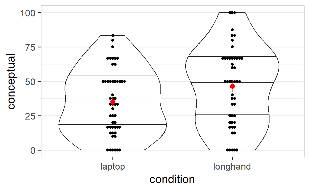
Figure 6.2: Conceptual memory scores from Mueller and Oppenheimer (2014). This plot combines individual data points in black with means in red.
Before looking at the figure, we see that we got a status message in the console, "No summary function supplied, defaulting to `mean_se()`". This message is always shown when using stat_summary() without additional argument and can be safely ignored (i.e., it just indicates that the red point shows the mean and the red error bars show the standard error).
The plot itself does not show anything unusual. The plot just reinforces the previous descriptive results: The mean memory score, but also the three displayed quantiles, are larger in the longhand than in the laptop condition. Taken together, the descriptive analysis suggests that there is nothing preventing us from running the inferential analysis and that there might be a difference such that conceptual memory scores might be larger in the longhand condition.
6.3.3 Inferential Analysis
The inferential analysis of the conceptual scores uses exactly the same call as our previous analysis, only with a new data set, mo2014_e2a.
mc_mo <- aov_car(conceptual ~ condition + Error(pid), mo2014_e2a)
#> Contrasts set to contr.sum for the following variables: condition
mc_mo
#> Anova Table (Type 3 tests)
#>
#> Response: conceptual
#>      Effect    df    MSE      F  ges p.value
#> 1 condition 1, 97 688.89 4.77 * .047    .031
#> ---
#> Signif. codes:
#> 0 '***' 0.001 '**' 0.01 '*' 0.05 '+' 0.1 ' ' 1
Looking at the ANOVA table of the results shows that the \(p\)-value is smaller than .05; the analysis reveals a significant effect of condition. This indicates that this data provides evidence against the null hypothesis of no difference between the note taking conditions. Consequently, we would be justified in saying that the data provides evidence for a difference.
To make it easy to detect a significant result, afex – like most statistical software tools – indicates a significant effect with \(p < .05\) with one * next to the \(F\)-value. In case of a significant result with \(p < .01\), this is indicted by two **. In case of a significant results with \(p < .001\), this is indicated with three ***. In case the effect is not significant, but \(p < .1\), a + is shown at that position (however, this does not indicate that the data is almost significant).
We can use afex_plot() in the same way as above to produce a results figure based on the estimated model, with the individual data points shown in grey in the background.
afex_plot(mc_mo, "condition")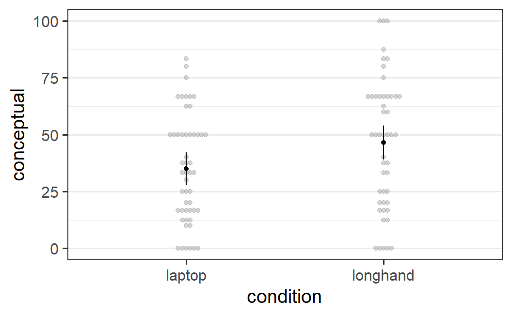
Figure 6.3: afex_plot() figure for the conceptual memory scores from Mueller and Oppenheimer (2014, Experiment 2) that show a significant difference between the two note taking conditions.
We can also use emmeans() to obtain the estimated marginal means:
emmeans(mc_mo, "condition")
#>  condition emmean   SE df lower.CL upper.CL
#>  laptop      35.0 3.68 97     27.7     42.3
#>  longhand    46.5 3.79 97     39.0     54.0
#>
#> Confidence level used: 0.95
Likewise, we can use emmeans() in combination with `pairs() to obtain the estimated difference between the two conditions:
emmeans(mc_mo, "condition") %>%
  pairs()
#>  contrast          estimate   SE df t.ratio p.value
#>  laptop - longhand    -11.5 5.28 97  -2.184  0.0314
If we were to report this study in a research paper, we could do so in the following way:
Figure 6.3 shows the conceptual memory scores from Mueller and Oppenheimer (2014) and suggests that conceptual memory is somewhat better in the longhand compared to the laptop note taking condition. In line with this visual impression, an ANOVA on the conceptual memory scores indicated a significant effect of note taking condition, \(F(1, 97) = 4.77\), \(p = .031\). The mean scores in the longhand condition (mean = 46.5, SD = 28.9) were significantly larger than the mean scores in the longhand condition (mean = 35.0, SD = 23.5), with a difference of 11.5 (SE = 5.3). This suggests that the type of note taking during lectures, either with a laptop or in loghand format, might have an effect on the conceptual memory for the content of the lectures.
6.4 Conceptual Memory Scores from Mueller and Oppenheimer (2014) Experiment 1
As discussed above, the two data sets looked at so far are both direct replications of Mueller and Oppenheimer (2014)'s Experiment 1, a data set which we have not yet discussed. Consequently, we are now re-analysing this data set, Mueller and Oppenheimer (2014)'s Experiment 1. This data is also available from the OSF.
The following code snippet prepares the data using the same strategy as for Experiment 2 shown above. As party of this preparation, the code excludes the one participant also excluded by Mueller and Oppenheimer (2014). The code ends up with the same number of participants as reported by Mueller and Oppenheimer (2014) (see here).
mo2014_e1 <- read_csv("data/Study 1 abbreviated data.csv")
#> Rows: 66 Columns: 22
#> ── Column specification ────────────────────────────────────
#> Delimiter: ","
#> dbl (22): participant, LapLong, whichtalk, threeGR, Wcou...
#>
#> ℹ Use `spec()` to retrieve the full column specification for this data.
#> ℹ Specify the column types or set `show_col_types = FALSE` to quiet this message.
mo2014_e1 <- mo2014_e1 %>%
  filter(participant != 63) %>%
  mutate(
    pid = factor(participant),
    condition = factor(LapLong,
                       levels = c(0, 1),
                       labels = c("laptop", "longhand"))
  ) %>%
    mutate(
    factual = factualindex / perfectfactindexscore * 100,
    conceptual = conceptualindex / perfectconceptindexscore * 100
  ) %>%
  select(pid, condition, factual, conceptual)
glimpse(mo2014_e1)
#> Rows: 65
#> Columns: 4
#> $ pid        <fct> 1, 2, 3, 4, 5, 6, 7, 8, 9, 10, 11, 12, …
#> $ condition  <fct> longhand, longhand, longhand, laptop, l…
#> $ factual    <dbl> 50.00000, 52.38095, 92.85714, 73.80952,…
#> $ conceptual <dbl> 50.00000, 50.00000, 66.66667, 83.33333,…
mo2014_e1 %>%
  count(condition)
#> # A tibble: 2 × 2
#>   condition     n
#>   <fct>     <int>
#> 1 laptop       31
#> 2 longhand     34
We can then run the same analysis as for the other data sets:
mc_mo1 <- aov_car(conceptual ~ condition + Error(pid), mo2014_e1)
#> Contrasts set to contr.sum for the following variables: condition
mc_mo1
#> Anova Table (Type 3 tests)
#>
#> Response: conceptual
#>      Effect    df    MSE    F  ges p.value
#> 1 condition 1, 63 530.96 2.46 .038    .122
#> ---
#> Signif. codes:
#> 0 '***' 0.001 '**' 0.01 '*' 0.05 '+' 0.1 ' ' 1
The results do not show a significant effect of note taking condition, \(F(1, 63) = 2.46\), \(p = .122\). This is a somewhat surprising result, because Mueller and Oppenheimer (2014) did report a significant effect with \(p = .046\). The reason for this difference is that they used a different statistical analysis than the ANOVA reported here, a mixed-effects model (for an introduction, see Singmann and Kellen 2019).
Whether their analysis is more appropriate than the ANOVA analysis performed here, is not something that we can discuss here in detail. Mixed models are a more advanced statistical procedure for which the appropriate specification is not always straight forward. In any case, the fact that our very sensible analysis shows a clearly non-significant difference suggests that the results of their Experiment 1 are not as clear cut. In other words, we have a situation where two seemingly sensible analysis strategies lead to different qualitative results. This indicates that the evidence for a difference in the population is not very strong.
If we plot the data using afex_plot() the visual impression is in line with the statistical one. Even though the observed difference is in the same direction as for Experiment 1, the difference appears smaller. We can also see that three participants in the longhand conditions have the overall lowest conceptual memory scores, even though the mean of the longhand condition is larger than the mean in the laptop condition.
afex_plot(mc_mo1, "condition")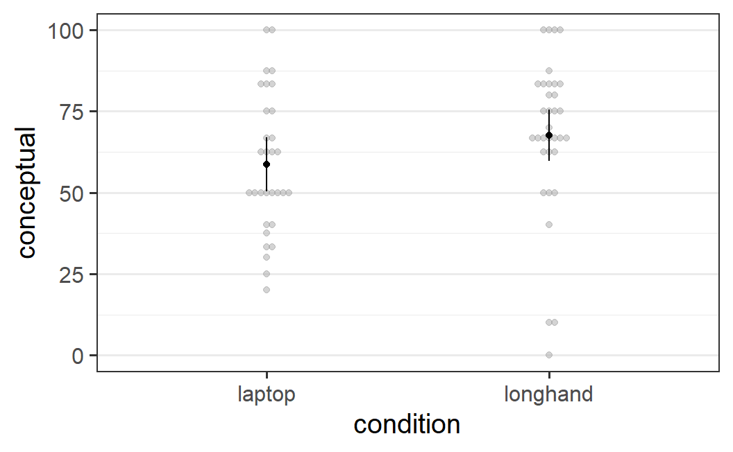
Figure 6.4: afex_plot() figure for the conceptual memory scores from Mueller and Oppenheimer (2014, Experiment 1). The ANOVA shows no significant difference between the two note taking conditions.
We can also use the combination of emmeans() and pairs() introduced before to get the estimated difference. This shows that the memory benefit for longhand note taking in this experiment is a bit less than 9 points, rounded to 9.0 points.
emmeans(mc_mo1, "condition") %>%
  pairs()
#>  contrast          estimate   SE df t.ratio p.value
#>  laptop - longhand    -8.97 5.72 63  -1.567  0.1220
Overall, the results from Mueller and Oppenheimer (2014)'s Experiment 1 look similar but also different to the results from their Experiment 2. The results are similar because the observed conceptual memory benefit for the longhand condition is 9.0 points for Experiment 1 and was 11.5 points Experiment 2. The results are different because the effect was only significant for Experiment 2, but not for Experiment 1.
One possible reason for this difference in inferential outcome (i.e., significant versus not significant) could be the difference in sample size. Each condition in Experiment 1 consisted of around 30 participants, whereas each condition in Experiment 2 consisted of around 50 participants. One general rule for NHST is that for a fixed observed effect, the study with the larger sample size will have a lower \(p\)-value. The reason for this behaviour of NHST is something that makes intuitive sense, the larger the sample size the more representative the observed effect becomes for the effect in the population. In the limit when we have observed all participants in the population (i.e., sample = population), the effect of the sample is identical to the effect in the population.
6.5 Overview of Experiments Investigating Longhand versus Laptop Notetaking During Lectures
Let's try to sum up what we have learned about different types of note taking for memory performance. In the previous chapter (Chapter 5, we have seen that the overall memory performance in the study of Urry et al. (2021) is slightly and non-significantly higher after taking notes with a laptop compared to longhand format.
In this chapter, we have been concerned with the conceptual memory scores only, which are one part of the overall memory scores. The reason for focussing on the conceptual memory scores was doing so was based on Mueller and Oppenheimer (2014). They argued that "[l]aptop use facilitates verbatim transcription of lecture content because most students can type significantly faster than they can write" (p. 1160). Furthermore, "[p]revious studies have shown that detriments due to verbatim note taking are more prominent for conceptual than for factual items" (p. 1160). Consequently, they expected that note taking with a laptop will lead to reduced conceptual memory compared to note taking in longhand format.
When looking at only conceptual memory scores and only considering the experimental design introduced above, we have data from three basically identical studies: Experiments 1 and 2 of Mueller and Oppenheimer (2014) and the experiment of Urry et al. (2021).
As we have shown above, the data of Urry et al. (2021) showed a slight and non-significant memory advantage in the laptop compared to the longhand condition (difference of 3.5 points). Experiment 1 and 2 of Mueller and Oppenheimer (2014) show the opposite results pattern, a benefit for longhand compared to laptop note taking of around 10 points (Experiment 1 = 9.0 points, Experiment 2 = 11.5 points). In our reanalysis the observed effects are quite similar across these two experiments of Mueller and Oppenheimer (2014), but it is only significant for Experiment 2 and not for Experiment 1.
If we consider the results from the three experiments together, there is limited evidence for an overall effect of the type of note taking on conceptual memory. Whereas Mueller and Oppenheimer (2014) clearly suggest that note taking in longhand format is better, Urry et al. (2021) descriptively observe the opposite pattern with roughly the same number of participants (total N = 142) as Experiments 1 and 2 of Mueller and Oppenheimer (2014) combined (total N = 164).
What does this mean for the research question that the type of note taking matters for conceptual memory? There are three different situations that could be responsible for the inconsistent results. Each of these different situations has a different consequence for the research.
The first possibility is that there is an effect of the type of note taking on conceptual memory in the population. In this situation, the study of Urry et al. (2021) produced a false negative result; a non-significant effect in the sample when in reality there is an effect in the population – that is, in reality the null hypothesis is false. As NHST results are always probabilistic, such a false negative result can always happen due to random chance (i.e., researchers can just get unlucky). Other possible reasons for this possibility could be (a) an error during data collection or data handling (e.g., condition codes are incorrectly assigned to participants) or (b) some sort of experimenter demand effect. An experimenter demand effect can happen if the person performing the data collection knows about the hypothesis and in which condition a participant is and influences the participant subtly in a specific direction. This influence can happen unknown to both the experimenter and the participant. For example, if most of the students performing the data collection did not believe in the hypothesis that the type of note taking had an effect they could have acted in a way that made the task more difficult for participants in the longhand condition.
The second possibility is that there is that there is no effect of the type of note taking on conceptual memory in the population. In this situation, the study of Mueller and Oppenheimer (2014) produced false positive results; a significant effect in the sample when in reality there is no effect in the population – that is, in reality the null hypothesis is true. Again, such an outcome can occur purely due to chance. However, the more studies in a row show a significant effect, the less likely such a chance outcome is at least in theory (because in our reanalysis the results from Experiment 1 changed from significant to non-significant, this is not a very strong argument here). Other possible reasons for this possibility are the same as above, an error in the studies or experimenter demand effects. For example, it is quite likely that the researchers performing the data collection for Mueller and Oppenheimer (2014) believed in the hypothesis that note taking with a laptop leads to worse memory than note taking in longhand format. Therefore, they might have acted in a way that made the task more difficult for participants in the laptop condition.
The third possibility is that neither of the results is a false positive or false negative, but both correctly reflect the underlying population. In this situation, there are two different populations from which the two different papers have sampled their participants. For example, the data collection of Mueller and Oppenheimer (2014) must have taken place in 2013 or earlier. It is conceivable that the participants at that time were still used to taking most of their lecture notes in longhand format and thus might have performed better in the format they are more used to. In contrast, the data collection of Urry et al. (2021) took place in spring 2017 and students at that time might have been more used to note taking with a laptop thus removing a potential benefit of note taking in a longhand format. In other words, whereas there might have been a difference in population earlier this difference might have disappeared by now where most people use their laptops everyday now.59
In the absence of any additional data or studies, it is very difficult to decide between these three possibilities. Many researchers seem to put more weight on the first study that published a study using a specific experimental task than the following replication studies. In this mindset, we would still believe that the effect of Mueller and Oppenheimer (2014) "is real" whereas the results of Urry et al. (2021) must be a fluke. However, it is difficult to see a logical argument for such a position. On the other extreme is a position held by some researchers that if there is a failed replication of a study, this means that there must have been something wrong with the original study. Again, this position does not seem logically justifiable. Whereas a failed replication clearly weakens the claims made in the original study, it does not mean anything is necessarily wrong with it.
Before deciding what we should believe, let's consider in detail the consequences if the first possibility described above is actually true. As a reminder, this possibility is that Urry et al. (2021)'s results are a false negative result and in reality there is a difference in the population between the two note taking conditions on the conceptual memory scores. But what does this outcome mean for our research question? For this, we need to circle back to the two epistemic gaps discussed in Section 1.3. If we knew for sure that there is an effect of note taking on the population than the second epistemic gap would not apply any more. However, the first epistemic gap would still apply.
Only because we knew that there were a benefit of note taking in longhand compared to laptop format in the experimental task developed by Mueller and Oppenheimer (2014), this does not mean that such a benefit always occurs for all lectures and for all people. For example, the experiment only used a rather short video lectures of around 15 minutes in length. Would such a benefit also occur for longer lectures? Likewise, does this effect only appear for the relatively well educated participants of the original study or really apply to the whole population of students? Another potential issue is how long the memory benefit holds. In the experiments considered here, the memory task followed around thirty minutes after the lecture. Mueller and Oppenheimer (2014) addressed this question in their Experiment 3, where testing took place roughly one week after the virtual and still found a longhand memory benefit. However, this result has to the best of my knowledge as of yet not been replicated.
What this list of open questions shows is that even in the best case scenario in which we knew that the failed replication were not a problem, the implications from the statistical result for our research question would still be limited. As discussed in detail in Section 1.3.1, the largest problem for a strong inference from any statistical result is the underdetermination of theory by data. Only because we find a specific pattern with one specific operationalisation, this does pattern generalises to all instances for which we hope our research question applies. One of the most important – and perhaps most difficult – tasks researchers is to not fall into the trap and interpret a significant \(p\)-value as an answer to our research question. It only is one piece of evidence in the research process.
In sum, the results suggests that if there is a benefit of a particular type of note taking on conceptual memory, it is not easy to detect. The available data does not suggest that everyone should ditch their laptop for paper and pencil. These results should also not be used to justify prohibiting students from using their laptops during lectures. If researchers and educators feel that this is an important research and real-life question, they need to provide stronger evidence.
6.6 Summary
In this chapter, we have discussed three things. Firstly, we have used the tidyverse and prepared the data from two Experiments of Mueller and Oppenheimer (2014) for analysis. We have seen that such a data preparation often not only requires the necessary tidyverse skills, but also knowledge of the data set. As part of this data preparation, we have discussed the importance of performing coherence checks to ensure the data matches our assumptions. Only when we have assured ourselves that the data is okay we can go ahead and perform the statistical analysis.
Secondly, we have used afex::aov_car() and re-analysed three data sets using NHST. These three data sets shared the same structure, one continuous dependent variable and one categorical independent variable with two levels, and we could therefore use the ANOVA approach introduced in the previous chapter for the analysis. As part of this analysis, we have also created results figures using afex_plot() and performed follow-up analyses using emmeans(). We could see that once the data set is in the correct format, estimating the statistical model and obtaining the \(p\)-value and performs additional analyses and plotting is relatively straight forward.
Thirdly, we have discussed what we learn from the three different experiments for the research question on how different types of note taking during lectures affect the conceptual memory for the lecture content. We have seen that despite the results from Mueller and Oppenheimer (2014) that suggests that note taking in longhand format provides a memory benefit compared to note taking with a laptop, the overall conclusion is not that clear. One problem is that the replication of Urry et al. (2021) questions whether the original pattern is a genuine effect that holds in the population. The other problem is that even if the results of Mueller and Oppenheimer (2014) would reliable replicate, that would not provide a conclusive answer to the general research question. Only because we find a results with one operationalisation, this does not mean it holds for the underlying research question. In the reality of research, the epistemic problems discussed in Chapter 1 cannot be ignored.
The overarching goal of this chapter was to paint a realistic picture of what we can learn from a significant result. One reality of research practice is that a significant results is generally what researchers are looking for. If a results is significant we are happy – our experiment "has worked" and we can publish it. If the result is not significant we are unhappy, because we generally have problems publishing our results. Whereas this might be the reality of research practice, the significant \(p\)-value is not actually the end goal. "The mistake is to think that statistical inference is the same as scientific inference." (Rothman, Gallacher, and Hatch 2013, 1013). In other words, even if we find a significant \(p\)-value what we can learn from a particular study is always limited. Likewise, if we use an established task or study an established phenomenon, finding a non-significant result can also be of major interest.
The focus on whether or not a \(p\)-value is significant has created a situation that in many domains the published literature paints a picture that it is easy to obtain a particular result. However, the reality is that this is often not the case, simply because researcher do not publish the failed attempts. In sum, please do not confuse the \(p\)-value with the answer to your research question.