1 Role of Statistics in the Research Process
In this book we are concerned with experimental psychology, in particular the statistical analysis of experiments in psychology and related disciplines such as language science, behavioural science, cognitive science, or neuroscience. The order expressed in the previous sentence – science first and statistical analysis second – is one of the overarching principles with which we will think about statistics. Whereas the goal here is to introduce the concepts and techniques required to perform a statistical analysis of (mostly experimental) data, the perspective taken is that a statistical analysis can only be performed or understood within the scientific context it takes place in.
One consequence of this perspective is that the start point of any statistical analysis needs to be a specific and clear research question. In the case in which both data collection and analysis is guided by such a research question, a statistical analysis is generally an indispensable part of the research process. As we will describe in more detail in this and the coming chapters, statistics is the tool that allows us to draw inferences that go beyond the data we have observed. This ability to generalise is what allows us to connect experimental results with the research questions and underlying theories. In sum, the statistical techniques introduced in this book can provide meaningful and scientifically helpful answers when the data is collected and analysed with a clear research question in mind.
1.1 The Research Process
One way to describe the research process in psychology and related sciences is in terms of four interrelated steps: the research question, the operationalisation of the research question and the data collection, the statistical analysis of the data, and finally the communication of the results. Let us explain these steps in more detail.
Any research should begin with a research question. For the disciplines considered here this is often a theory or hypothesis about human behaviour or the human mind. For example, a widely accepted idea in decision making and behavioural science is that people exhibit loss aversion – the displeasure resulting from losing £10 is stronger than the pleasure derived from winning £10. We will look at this example research question, whether there is evidence for the idea of loss aversion, in more detail in this chapter. What the example already shows is something that is common for research questions – it contains a general statement that involves not directly observable quantities (such as pleasure or displeasure).
Not all research questions are as general as the question of whether there is loss aversion. In fact, many research questions are a lot more specific or more applied. For example, in many applied domains an important question is whether a specific intervention – such as a new therapeutical procedure or a workplace training – is better than no intervention or an already existing one.
Sometimes, the researcher just wants to find an answer to a specific issue that had come up in a previous study. As a concrete example, consider Hinze and Wiley (2011) that addresses a specific question concerning the testing effect. The testing effect describes the now well established phenomenon that testing of newly learned materials (e.g., self-tests or quizzes) leads to better memory than additional studying (e.g., re-reading) (Roediger and Karpicke 2006). What Hinze and Wiley (2011) noticed was that at that time most research on the testing effect only used limited ways of implementing testing, such as multiple choice tests or open-ended questions. To see whether the phenomenon was more general, their research question was whether the testing effect also occurred for another type of testing, fill-in-the blank tests (i.e., sentences from the learned materials were shown with some words missing that needed to be filled in). The results showed that fill-in-the blank tests were not more effective than mere re-reading and did not show a genuine testing effect (at least not one that goes beyond the specific words that had to be filled in). Thus, fill-in-the-blank is not a testing (or) strategy that is as effective as testing types that require more involved processing of the materials (e.g., open ended questions).
The next step in the research process is the transformation of the research question into an empirical and statistical hypothesis. We will call this step operationalisation. That is, instead of talking about abstract ideas or research questions, we need to concretely decide which study to run. We need to find tasks or other measures (e.g., questionnaires) that allow us to collect data that addresses our research question. An important part of the operationalisation is the specification of relevant variables. We can understand variables as dimensions, features, or characteristics on which individuals or situations can differ. For example, relevant variables for loss aversion are the magnitude of a potential loss or gain and the intensity of resulting pleasure or displeasure (e.g., as measured from a questionnaire). For the testing effect, relevant variables are the type of additional learning (e.g. re-reading versus multiple choice testing) and the final memory performance.
As we can see from the example of the testing effect, sometimes it appears difficult to separate the research question from its operationalisation. In this case, the research question is tied to a specific aspect of the operationalisation (i.e., how testing is implemented). However, even with a concrete research question there are always other aspects of the study that require further operationalisation (e.g., what is our measure of learning?). As the example of loss aversion shows, some research questions are very general. Consequently, there are a multitude of possible studies that can be performed to investigate one research question. However, for any specific study a researcher needs to decide on one specific study design. What exactly are the tasks and measures we are using to investigate the question we are interested in?
The traditional view of the research process – known as the hypothetico-deductive method – is that during the operationalisation step, researchers derive an empirical prediction that tests their theory. In other words, the theory coupled with the operationalisation predicts a specific outcome (the empirical prediction), that needs to occur if the theory is true. For example, as we will discuss in detail below, loss aversion predicts that people should be unwilling to gamble money if the chance of losing a specific amount of money is equal to the chance of winning the same amount of money (because losing that amount hurts more than winning that amount). According to the traditional view, if this predicted outcome were not to occur, we would learn that the theory is false. Furthermore, if the predicted outcome were to occur, this would not entail that the theory is necessarily true, but it would provide support for the theory. However, as we will see below (Section 1.3.1), in reality we generally learn less than that prescribed by the idealised form of the hypothetico-deductive method.
Research practice often diverges from this idealised view of the research process (e.g., Haig 2014). Not in all cases is there one clear prediction or specific theory that is tested. Researchers might compare multiple theories with diverging predictions, only have a vague hypothesis instead of a fully fledged theory from which more than a single prediction follows, or they might simply be curious about what happens in a specific situation. For example, in Hinze and Wiley (2011), the research question was if the fill-in-the blank test would show the same testing effect as other testing procedures. None of the possible results, even the complete absence of a testing effect for this type of testing, would have provided evidence against testing effects in general. The goal of the research was not to confirm or disconfirm the testing effect. Instead, the goal was to test the generality of the testing effect. Consequently, it does not seem appropriate to say operationalisation always involves making specific empirical predictions. However, even in the absence of a specific empirical prediction, the operationalisation must result in an empirical hypothesis relating two or more of the variables that are part of the research design to the research question.1 The final step of the operationalisation is the data collection.
Once the research question has been operationalised and the corresponding data is collected, it is time for the statistical analysis. Generally, the statistical analysis answers one specific question: Does the data provide evidence for the empirical hypothesis derived from the research question? The remainder of this book will show in detail how to perform statistical analyses for common study designs and how to interpret the results in light of the research question and operationalisation.
Once the data is sufficiently analysed, we have reached the final step of the research process, we need to communicate the results (this step is also known as dissemination). There are different forms of dissemination depending on your goal and audience (e.g., scientific journal article, dissertation report, conference presentation, or a press release). Whereas the different forms differ in the amount of detail and background that is provided, they all need to provide a truthful and comprehensive account of the whole research process: What is the research question? How was it investigated (i.e., describe the operationalisation)? What are the results? What does this mean for the research question? Often, the difficult problem to solve during this step is to provide a comprehensive and truthful account but in a succinct manner. One important tool for doing so is through graphical means – pictures of the results. Consequently, in this book we will discuss both how to present statistical results in a text and how to create appropriate graphs.
Whereas this abstract overview leaves out some important things that are also part of research – such as where research questions come from – it shows three important things.
The primacy of the research question. The research question determines the operationalisation and thus which data is collected. The research question also determines the statistical analysis, but indirectly; the research question determines the empirical hypothesis which is then tested in the analysis.
The statistical analysis is not directly connected to the research question. The statistical analysis is performed on the operationalisation of the research question, but not on the research question itself. What this means is that the statistical analysis itself cannot directly inform us about the research question. In other words, we cannot statistically test the research question. Instead, statistics can only tell us something about a specific operationalisation. Whether or not this allows strong inferences about the research question depends on the operationalisation. And as shown in the following example, an important part of the scientific discourse is to argue whether certain operationalisations allow one to address specific research questions. However, this is generally not a statistical question.
Statistics is not the end goal of the research. Instead, the end goal is usually a written communication of the research. In most cases, the statistical analysis is an indispensable part of this communication in that it can provide evidence for or against a specific empirical hypothesis. However, to understand the full meaning and implications of a particular statistical result, it is important to know its context – the research question and its operationalisation. It is the task of the researcher to communicate this context when communicating the research. Without the context, the impact and meaning of a statistical result is severely limited.
1.2 Example: The Psychology of Loss Aversion
To get a better understanding of the research process and the problems that can arise in it, let us consider in detail a concrete example of a research question and how it can be investigated empirically. Specifically, let us return to the example of loss aversion. Loss aversion is one of the assumptions underlying prospect theory (Kahneman and Tversky 1979), a mathematically formalised theory combining cognitive psychology with economic theory.2 The concise description of loss aversion is that "losses loom larger than gains" (Kahneman and Tversky 1979, 279). As described above, loss aversion means that the negative feeling associated with a loss of a certain amount of money is larger than the positive feeling associated with a gain of the same amount. For example, loss aversion predicts that the displeasure or pain from losing £10 is larger than the pleasure or joy from winning £10.
We can see that loss aversion is a theoretical statement involving latent - that is, unobservable - quantities such as negative or positive feelings (i.e., displeasure versus pleasure). We can ask people how they feel, but we cannot easily observe feelings without asking. In psychology, we generally call unobservable theoretical concepts constructs. So how can we test whether people indeed show loss aversion if we cannot directly observe the constructs that form the core of it?
One possibility for testing the hypothesis that individuals show loss aversion is hinted at above. We could either give people a certain amount, say £10, or take it away from them, and then ask them how they feel. This procedure runs into at least two problems. First, it is clearly ethically unacceptable to perform an experiment that consists of taking £10 away from our participants. Second, even if we were to overcome the ethical problems (e.g., by first giving participants an endowment and only taking money away from that endowment) there would still be the problem of how to measure the feelings associated with the two events.
One way to avoid the ethical problem of taking away money from participants is to ask them to imagine how they would feel if they lost or gained a certain amount of money. Even though it is not certain whether this imagined feeling corresponds to the actual feeling the participants would have when actually losing or gaining this amount, this procedure is commonly used. For example, McGraw et al. (2010) asked their participants to imagine that they would play a single game with a 50% chance of losing $200 and a 50% chance of winning $200 (e.g., flipping a coin and if it comes up heads you win $200; otherwise you lose $200). They then asked participants to imagine how they would feel after either of the two outcomes. They identified two different ways to ask this question, both of which are shown in Figure 1.1 below (McGraw et al. 2010). The first possibility, a bipolar scale, is shown in the upper part. On this response scale participants in the loss condition respond on the left side of the scale and participants in the gain condition respond on the right side of the scale. To compare the ratings, they measured participants' responses as the absolute distance of the rating from the neutral point "No Effect" (i.e., "Small Positive Effect" would be treated as the same intensity as "Small Negative Effect"). The second possibility is shown in the lower part of Figure 1.1 and shows a unipolar intensity scale. On this scale, participants in both conditions provide their response on the same scale and only rate the intensity of their displeasure or pleasure.
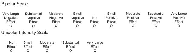
Figure 1.1: Example of two different scales for measuring feelings after a potential gain and loss. The upper part shows a bipolar scale in which losses receive a rating on the left side (of No Effect) and gains receive a rating on the right side. The lower part shows a unipolar scale in which the intensity for both losses and gains are given on the same scale. Image adapted from McGraw et al. (2010).
Before reading on, take a moment and ask yourself if you believe the two scales shown in Figure 1.1 make a difference to whether or not participants show loss aversion. Or put differently, can you think of a reason why it matters how we ask for participants' feelings after a loss or gain? And if there were a difference, on which scale would you expect it to be more likely that loss aversion occurs?
To investigate the question of whether there is loss aversion for both scales, McGraw et al. (2010) asked half of their participants to use the bipolar scale and the other half to use the unipolar scale to rate their feelings after the imagined loss and gain of $200. With this data in hand, they then compared the feeling ratings for imagined losses and wins for each of the two conditions. Their results showed that it indeed matters which scale is used. For the bipolar scale, there was no evidence for loss aversion. The feeling ratings for gains and losses were approximately equal at around 3.4 (where 1 = No Effect and 5 = Very Large Effect). However, when using the unipolar scale, they found evidence for loss aversion. In the loss condition, participants reported a stronger feeling on average (at around 3.6) compared to the gain condition (at around 3.1).
McGraw et al. (2010) explain the results in terms of relative versus absolute feeling judgements. For the bipolar scale, people first judge the valence of the feeling – that is, whether it is good or bad – to determine the side on which they have to provide their response. Once this is done, they only then judge the intensity of the feeling. However, as the intensity judgement follows the valence judgement, they make this intensity judgement only by comparing against other feelings of the same valence. More specifically, McGraw et al. (2010) assume that in the loss condition, the loss is only compared against other negative events. Similarly, in the gain condition, the gain is only compared with other positive events. In other words, for the bipolar scale, participants only make a relative judgement of intensity which cannot be compared for loss and gains. Consequently, they argue that the results from the bipolar scale are not helpful in answering the question of whether or not there is loss aversion.3
For the unipolar scale, McGraw et al. (2010) argue that the judgement of feeling intensity is not preceded by a valence judgement. Therefore, people use an absolute judgement of feeling, comparing it with both negative and positive feelings. Consequently, this data, which shows a pattern in line with loss aversion, is helpful for the question of whether or not there is loss aversion. Overall they conclude that their study provides evidence for loss aversion, because it appears when using the unipolar scale.
What the results of McGraw et al. (2010) show is that seemingly minor differences in the operationalisation of a research question can have a tremendous effect on the results. In line with this, it is perhaps not too surprising that this operationalisation for investigating loss aversion – asking participants about their feelings – is not very common. Below we will discuss alternative operationalisations.
And whereas McGraw et al. (2010) provide an explanation for the results, it is an explanation that might have been difficult to come up with before having seen the data. This inability to predict the effects of the response scale on the results has potential consequences that are further reaching. If we take their results seriously and generalise them to other domains, we might conclude that whenever we are interested in participants' feelings it matters whether we use bipolar or unipolar scales. One could even go another step further and say that whenever we use subjective rating scales, the type of the scale could have an unintended effect on the results. Because of this, it is often a good idea to try to find an operationalisation of research questions that do not only involve subjective rating scales, but other types of responses such as choices, response times, or more complex behaviour.
1.2.1 Evidence for Loss Aversion: Lotteries
A different operationalisation for testing loss aversion is to compare choices across different risky choices, lotteries, or gambles (these terms can be understood interchangeably here), a common experimental paradigm in decision making and behavioural economics. A lottery in this context consists of different options, each of which is associated with one or multiple outcomes, from which the participant has to choose one.
The simplest type of lotteries are ones consisting of only one option. In this case, participants can only decide whether to accept or reject the lottery. For example, evidence for loss aversion can be found in the lotteries used by Battalio, Kagel, and Jiranyakul (1990). One of their lotteries (their Question 15) was:
Would you play the following gamble:
A 50% chance of losing $20 or a 50% chance of winning $20.
Participants then had to decide whether to accept or reject the lottery.4 43% of participants accepted this lottery.
It is not only participants in the experiment of Battalio, Kagel, and Jiranyakul (1990) who dislike symmetric 50-50 lotteries. The following clip from the YouTube channel Veritasium, also observes this in random people from the street.
So how do the result of Battalio, Kagel, and Jiranyakul (1990) provide evidence for loss aversion? The evidence comes from the fact that participants are more likely to reject the lottery than to accept it (i.e., the acceptance rate is below 50%). What is important about this lottery is that it is a symmetric 50-50 lottery. That is, the magnitude of the potential loss was equal to the magnitude of the potential gain and both possible outcomes appear with equal probability of 50%.5 Remember that loss aversion means disliking a loss more than liking a gain of the same magnitude. A symmetric lottery is exactly such a situation. The fact that participants are more likely to decline to participate in a symmetric lottery is therefore very much in line with loss aversion.
One problem with the results of Battalio, Kagel, and Jiranyakul (1990) is that they only collected data from 35 participants which did not provide statistically compelling evidence for loss aversion. Whereas the data shows a descriptive pattern that is in line with loss aversion (i.e., below 50% acceptance of symmetric lotteries) this is not supported by a statistical analysis. More specifically, the statistical analysis does not provide support for the empirical prediction that the observed acceptance rate is below 50%.[a] It does descriptively look like this, but the evidence in the data is not enough to surpass the statistical criterion we use for judging the evidence. A fuller description of how we set a statistical criterion will come later.
More compelling evidence for loss aversion comes from a study by Brooks and Zank (2005). In their task, participants were asked to make a decision about more complex lotteries in which participants had to decide between two options. For example, one of the lotteries was the following:
Which option do you prefer?
A: A 25% chance of +£11, a 50% chance of £0, or a 25% chance of -£11.
B: A 25% chance of +£10, a 50% chance of £0, or a 25% chance of -£10.
We see that for each of the two options, there are two symmetric outcomes of the same magnitude. For both options A and B, there is a 25% chance of a loss and a 25% chance of a gain of the same magnitude (and with 50% probability participants neither lose nor gain anything). The difference between A and B is that for A, the magnitude of the potential loss and gain is larger by £1.
The notion of loss aversion makes an interesting prediction in this case. Participants should increasingly dislike a symmetric lottery the larger the potential outcomes are. For our lottery this means that if we dislike losing £10 more than liking gaining £10, this difference between dislike and liking should be larger if the potential outcomes are £11. In terms of empirical prediction this means that participants should be more willing to choose option B than option A in the lottery above.
In the study of Brooks and Zank (2005), each of 49 participants worked on around 50 lotteries that were all similar in structure to the lottery above. That is, for each of the two options there was a loss and gain of the same magnitude with the same probability (the third potential outcome was always smaller in magnitude than the loss/gain). As in the example lottery above, the difference between both options was always that the loss/gain magnitude for one option was £1 larger than for the other option. In line with the empirical prediction of loss aversion, participants chose the option with smaller magnitude of loss/gain in 63% of cases. And given the larger sample size in this study, the statistical analysis also supported the prediction that this 63% was larger than 50%.
So does this all show that there is such a thing as loss aversion? Results such as those from Brooks and Zank (2005) certainly appear to support this theoretical idea (see also Camerer 2005). And this also makes intuitive sense. Most people (me included) feel that symmetric lotteries are not really attractive and become increasingly unattractive with increasing magnitude (who really thinks flipping a coin for the chance of losing or winning say £100,000 sounds like a good idea?). However, as in the previous example, the evidence for loss aversion discussed here hinges on a particular operationalisation of the theoretical idea. From these results, we have not really learned that the magnitude of a loss or gain is the psychologically relevant factor in the minds of people. The only thing we have learned is that people dislike certain lotteries or options in lotteries. Can we find an alternative for this data pattern that does not involve loss aversion?
1.2.2 Alternative Explanation: Loss Aversion or Loss Seeking?
One clever alternative explanation for why it looks like there is loss aversion was provided by Walasek and Stewart (2015). In their study, participants were also presented with 50-50 lotteries. An example of one of their lotteries is shown in Figure 1.2 below. As shown in the figure, each lottery involved mixed outcomes, that is both gains and losses (i.e., -$18 and +$20 in the example). Furthermore, each lottery consisted of only one option, so participants only had to choose whether to accept and play a lottery or not. Finally, both possible outcomes always had a 50% probability of occurring. To make this logic clearer to participants, they were told that accepting the lottery shown in Figure 1.2 was equal to flipping a coin that has -$18 on one side and +$20 on the other side. Depending on which outcome came out on top, their money would change accordingly. If participants rejected a lottery, they neither lost nor won any money.
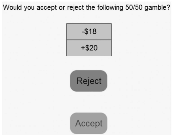
Figure 1.2: Screenshot of lottery task used to investigate loss aversion. This screenshot is from Walasek and Stewart (2015, Figure 1).
Before describing the study and its results in detail, let me first lay out the gist of the argument of Walasek and Stewart (2015). Among the lotteries participants saw in their study were some symmetric lotteries in which the potential loss was equal to the potential gain. For example, a -$12/+$12 lottery. If participants accepted most of these lotteries they would on average neither win nor lose money.
The clever manipulation of Walasek and Stewart (2015) was that across different conditions (i.e., groups of participants) they manipulated how attractive these symmetric lotteries were, relative to the other lotteries a participant saw. In one condition, there were many lotteries for which the potential loss was smaller than the potential gain, such as a -$12/+$20 lottery. That is, if a participant in this condition accepted most lotteries, they were likely to win money. In this condition the symmetric lotteries were therefore relatively unattractive. In another condition, there were many lotteries for which the potential loss was larger than the potential gain, such as a -$20/+$12 lottery. That is, if a participant in this condition accepted most lotteries, they were likely to lose money. In this condition the symmetric lotteries were therefore relatively attractive.
According to the original idea of loss aversion, the only thing that matters for a lottery is the absolute magnitude of its potential gains and losses so such a manipulation of relative attractiveness of symmetric lotteries should not have any effect whatsoever. However, the results of Walasek and Stewart (2015) showed that the manipulation mattered. In the condition in which the symmetric lotteries were relatively unattractive, participants only accepted them in 21% of cases, but in the condition in which the lotteries were relatively attractive, participants accepted them in 71% of cases. A statistical analysis supported the empirical prediction that the acceptance rates for symmetric lotteries differed across conditions. This is a results pattern that is in contradiction with the original idea of loss aversion.
In the next section we present the full details of the study of Walasek and Stewart (2015), before coming back to what this means for loss aversion and how it fits within the general theme of this chapter. If decision making research or behavioural economics is not your main interest, these details may not be super relevant to you, so it is okay if you do not understand all of it perfectly. However, because we use this study as an example in the next chapters it would be great to at least give it a cursory read.
1.2.2.1 Full Details of Walasek and Stewart (2015)
As in many experiments that fall within the cognitive domain, the study of Walasek and Stewart (2015) consisted of a series of similar trials in which participants had to do the same task (i.e., accept or reject the shown lottery). What differed across trials were the values of the two possible outcomes. For example, in one of the conditions of the experiment losses ranged from -$6 to -$20 in increments of -$2 (resulting in 8 different possible losses) and gains ranged from $12 to $40 in increments of $4 (resulting in 8 different possible gains). Across all trials for one participant in this condition, all possible losses were combined with all possible gains so that in total participants had to decide for \(8 \times 8 = 64\) lotteries whether they accepted or rejected it.
Within the 64 trials was a subset of trials that allowed the researchers to directly address the question of whether there is evidence for loss aversion.6 Whereas most of the lotteries shown to participants were asymmetric – that is, the potential loss differed numerically from the potential gain (as in the example of Figure 1.2) – a small subset of lotteries were symmetric. For these lotteries, the amounts for the potential loss were equal to the amount for the potential gain. More specifically, the symmetric lotteries were -$12/+$12, -$16/+$16, and -$20/+$20.
For the condition described above in which losses ranged up to -$20 and gains ranged up to +$40, the 191 participants accepted the symmetric lotteries only 21% of the time. 21% is descriptively below 50% indicating that participants indeed disliked these lotteries more than they liked them (i.e., they were overall more likely to reject than to accept the symmetric lotteries). Furthermore, a statistical analysis supported the empirical hypothesis (i.e., provided evidence that this pattern of results generalises beyond the current data). As described above, this result makes sense in light of loss aversion. When losing a certain amount of money is worse than winning the same amount of money, one should reject a symmetric lottery in which one is equally likely to lose or to win a certain amount of money.
The clever manipulation of Walasek and Stewart (2015) was that they included three further conditions in which they changed the range of possible outcomes. In addition to the -$20/+$40 condition discussed above, the 202 participants in the $-20/+$20 condition saw lotteries with losses ranging to -$20 and gains also ranging to +$20 only. Another group of 190 participants, the -$40/+$40 condition, saw lotteries with losses ranging to -$40 and gains also ranging to +$40. Finally, Walasek and Stewart (2015) also included a -$40/+$20 condition with 198 participants in which the losses ranged to -$40, but the gains only to +$20 (i.e., the complement to the -$20/+$40 condition). Importantly, in all conditions the number of possible outcomes for losses and gains was 8 (so the step size was either \(\pm\)$2 or \(\pm\)$4). Table 1.1 below shows the possible outcome for each condition
| Condition | ||||||||
|---|---|---|---|---|---|---|---|---|
| -$20/+$40: Gains | $12 | $16 | $20 | $24 | $28 | $32 | $36 | $40 |
| -$20/+$40: Losses | -$6 | -$8 | -$10 | -$12 | -$14 | -$16 | -$18 | -$20 |
| -$20/+$20: Gains | $6 | $8 | $10 | $12 | $14 | $16 | $18 | $20 |
| -$20/+$20: Losses | -$6 | -$8 | -$10 | -$12 | -$14 | -$16 | -$18 | -$20 |
| -$40/+$40: Gains | $12 | $16 | $20 | $24 | $28 | $32 | $36 | $40 |
| -$40/+$40: Losses | -$12 | -$16 | -$20 | -$24 | -$28 | -$32 | -$36 | -$40 |
| -$40/+$20: Gains | $6 | $8 | $10 | $12 | $14 | $16 | $18 | $20 |
| -$40/+$20: Losses | -$12 | -$16 | -$20 | -$24 | -$28 | -$32 | -$36 | -$40 |
As a consequence of this design, what changed across conditions was whether the symmetric lotteries were relatively good or relatively bad. To understand this, we need to look at the remaining asymmetric lotteries. In the -$20/+$40 condition discussed so far, there were more lotteries in which the possible gain was larger than the possible loss (e.g., a -$18/+$20 lottery) than lotteries for which the possible loss was larger than the gain (e.g., a -$20/+$18 lottery). Consequently, the symmetric lotteries were relatively bad (i.e., compared to the many lotteries in which the possible gain is larger than the possible loss). In the -$20/+$20 and -$40/+$40 conditions, the asymmetric lotteries were balanced. In half of the asymmetric lotteries the possible gain was larger than the possible loss, whereas for the other half the possible loss was larger than the possible gain. Consequently, the symmetric lotteries were neither relatively good nor relatively bad. Finally, in the -$40/+$20 condition the pattern was flipped with respect to the -$20/+$40 condition. There were only a few lotteries in which the possible gain was larger than the possible loss compared to the many lotteries for which the possible loss was larger than the gain. Consequently, the symmetric lotteries were relatively good.
So does it matter whether the symmetric lotteries are relatively good or not? Indeed it does. As a reminder, people were unlikely to accept the symmetric lotteries in the -$20/+$40 condition in which the symmetric lotteries were relatively bad. Participants in this condition only accepted 21% of the symmetric lotteries. In the -$20/+$20 condition in which the symmetric lotteries were neither relatively good nor relatively bad, participants accepted 50% of the symmetric lotteries. Similarly, in the -$40/+$40 condition participants accepted 45% of the symmetric lotteries. Finally, in the -$40/+$20 condition in which the symmetric lotteries were relatively good, participants accepted 71% of the symmetric lotteries. We can see that 71% is descriptively above 50%, indicating that participants here liked the symmetric lotteries more than they disliked them (i.e., they were overall more likely to accept than reject the lotteries). Furthermore, a statistical analysis supported the empirical hypothesis (i.e., provided evidence that this results pattern generalises beyond the current data).
1.2.2.2 What do the Results Mean for Loss Aversion?
What the results of Walasek and Stewart (2015) show, is that the choice pattern for lotteries are not always in line with the idea of loss aversion. Only in a context in which a symmetric lottery is relatively bad do we see evidence in line with the idea of loss aversion. If we are in a context in which a symmetric lottery is relatively good, we see the opposite pattern that one could term loss seeking. What does this mean for loss aversion? The original idea of Kahneman and Tversky (1979) that what matters is the magnitude of a loss or gain surely is not in line with the results of Walasek and Stewart (2015). Instead, Walasek and Stewart (2015) argue that what is relevant to determine the psychological impact of a gain or loss is the relative magnitude or rank of a possible outcome: Compared to other gains or losses I regularly experience, is this a large gain or large loss?
Before moving on and linking this example of the psychology of loss aversion to the general goal of this book, let us answer one last question. If what matters is the rank (as suggested by Walasek and Stewart (2015)) and not the magnitude of an outcome (as proposed by Kahneman and Tversky (1979)), why do we see evidence for an effect of magnitude in other studies investigating loss aversion that did not manipulate the context of gains and losses (e.g., Brooks and Zank 2005)? An answer to this question is provided by Stewart, Chater, and Brown (2006). They argue (and also provide empirical evidence) that in our daily lives we experience more small losses (e.g., buying something at the bakery) and more larger gains (e.g., the monthly salary). As a consequence, for a gain and loss with the same magnitude, the relative rank of the gain compared to all other gains is lower than the corresponding relative rank of the loss compared to all other losses. From this difference, we should generally observe a pattern consistent with loss aversion but for a different theoretical reason than proposed by Kahneman and Tversky (1979).
1.3 Epistemic Gaps: The Difference Between What we Want to Know and What we can Know
The goal of this chapter is to provide an introduction to the role of statistics in the research process. Why do we need statistics and what can it tell us about the research questions we are interested in? However, so far we have not talked much about statistics. Instead we have introduced an abstract concept of the research process and exemplified it with the example of loss aversion. What this example has tried to show is that even though we can find statistical evidence that supports our empirical hypothesis, this does not mean we have found an answer to our research question. The question of whether or not there is loss aversion is not a statistical question. The answer to the research question depends on whether we can rule out possible alternative explanations, for example, that it is the rank of a potential loss or gain that is important, rather than its magnitude. We nevertheless need statistics to help us determine whether our data provides support for the particular empirical hypothesis that operationalises our research question.
Let's put this more bluntly. If you do not yet know about statistics in detail, the application of statistical methods can appear like a magical machine that provides us with an answer to the research question we have. You throw your data in, turn the handle on the statistics machine, and get an answer to your research question out. Sadly, this image of statistics (not to mention needing a handle!) is false. The reason is that there are at least two epistemic gaps in the research process that prevent us from getting a straight answer to our research question. In this section we will introduce these gaps to ensure you can get a realistic image of the role of statistics in the research process.
Before explaining what an epistemic gap is, we need to take a step back and think about science in general. There are at least two different domains that constitute a scientific discipline. Firstly, we have the substantive content, what the science is about. For example, psychology is concerned with the human mind and behaviour. So one domain of psychology consists of theories about mind and behaviour (e.g., people exhibit loss aversion). But, just having theories is not enough. The problem is that there are many intuitively plausible but ultimately untrue theories [e.g., the idea that there are distinct "learning styles"; see Pashler et al. (2008)]. So the second domain constituting a science is research; systematic investigations of our research questions that provide us with evidence. This evidence allows us to decide which theories to believe and which theories to discard.
This perspective on science allows us to draw some conclusions about what this means for us as scientists. Firstly, it is important not to adopt theories too easily and early. As scientists we need to be natural sceptics. Instead of believing in a theory because it sounds compelling, we need to ask for the evidence first. We then need to evaluate the evidence and use this as the basis for the degree of our belief. For example, if there are a few independent studies that support a certain theoretical position (as in the case of loss aversion), it seems appropriate to consider a certain theoretical position as a possibility but also to consider alternative accounts (for example, the rank based account of Walasek and Stewart 2015). If the evidence is weaker, say only studies from the proponents of a theory, we should be even more cautious in the degree of belief we assign to a theory. And only if the scientific evidence is overwhelming should we be willing to treat a theory as approximately true. For psychology, there are not many theories for which the majority of researchers would agree that the latter criterion is reached (besides maybe operant and classical conditioning). As a consequence, in many cases, the best thing to do is to be honest and admit that the evidence is not sufficient to hold a strong theoretical position. For us scientists, this perspective also means that we need to be able to evaluate the evidence from the research in our area of interest. Doing so requires substantive knowledge about our research domain, but also the statistical knowledge that we will introduce in this book. Finally, it means that we need to be open to revising our beliefs in light of new evidence (as in the case of loss aversion and the results of Walasek and Stewart 2015).
As the last two paragraphs show, science is ultimately about evidence. What evidence do we have to support the theories in our field? As scientists we hope that statistics is a tool that helps us answer the question about evidence. And to some degree it does, but not as much as we would hope. We need to be aware of the epistemic gaps. Let us explain now what this means.
Epistemology is a branch of philosophy that is concerned with knowledge (e.g., what is knowledge, how do we know that we know) and justification (e.g., what is the reason I believe something) (for a philosophical overview see: Steup and Neta 2020). "Epistemic" is the corresponding adjective. Epistemology therefore, is the field that deals with philosophical questions at the core of science, for example, which theories should I believe based on the available evidence. An epistemic gap describes the difference between what we want to know and what we can actually know.7 Ideally, we want to know whether a theory or hypothesis is true. As we have already seen in the example above, in many cases even carefully designed experiments cannot unambiguously answer this question (e.g., before Walasek and Stewart (2015) the available evidence appeared to support 'loss aversion', but now we are not so sure about it). In the following, we will take a more abstract look at this question and discuss two general problems that further complicate this issue. What we can know is often quite different from what we would like to know. A competent application of statistics requires that one is aware of this problem and avoids over-interpreting the results from one's research.
1.3.1 Epistemic Gap 1: Underdetermination of Theory by Data
Above we have provided an example of a theoretical (or basic) research question (Is there evidence for loss aversion?). We have seen that answering the research question requires careful thinking about the operationalisation; how exactly should we set up a study to test this question? And once we have decided on one operationalisation, we have seen that we can find alternative explanations that can explain the results without making the assumptions of the original research question. In other words, even though the operationalisation was carefully chosen, it could not unambiguously answer our research question.
The fact that we could not compellingly answer the research questions despite employing a carefully chosen operationalisation is not a problem that is unique to our example. In contrast, an important insight from philosophy of science is that this is a problem of any empirical study. This issue is also known as underdetermination of theory by data or the Duhem-Quine thesis and always occurs if there is a difference between the research question and the corresponding operationalisation. And as we have seen in the examples, there essentially always is.
There are different aspects of underdetermination. The first has to do with the specification of the research question and its operationalisation. Research questions usually involve unobservable constructs – such as emotions (e.g., fear), memory, attention, comprehension, or learning – or vague phrases, such as "works better" or "improves". An empirical investigation of such questions however requires a precise specification and operationalisation. By going from the research question to the concrete operationalisation, there is no guarantee that the operationalisation captures the intended meaning of the research question.
For example, consider a test of a new therapeutic intervention compared with a standard one. Imagine we found that the new intervention decreased the self-reported discomfort of symptoms on a patient questionnaire more strongly than the old treatment, but did not reduce the number of sick days due to the disorder. Should we interpret this to mean that the new treatment "works better" than the old one? In some sense it does, but in another it does not. The problem is that the nuances that result from operationalising a research question concretely do not always align with the broad way in which we like to think about research questions.
At this point you might think this does not yet sound like such a big problem. We just need to define our research questions precisely enough and then we would be able to learn something about our research question. Sadly, this is easier said than done. The first problem is that it is often impossible to precisely define our research question, because we have not yet found a way to precisely define the constructs that are involved in it (this is known as the problem of coordination, (Kellen et al. 2021)). And in most cases, precisely defining these abstract constructs is not possible anyway.
For example, if you have the hypothesis that a specific emotion, say fear, is related to some behavioural pattern, say aggression, you run into the problem that there is not a generally agreed upon definition of either of these constructs. There probably exist questionnaires for measuring fearfulness and aggressive tendencies, but these questionnaires do not represent the corresponding constructs or a definition of them. If you were to ask a sample of participants to fill out these questionnaires and found that the scores of the participants in these two questionnaires are related, it would not allow you to conclude that fearfulness and aggression are related. The only conclusion that would be allowed is that fearfulness as measured with one questionnaire is related to aggression as measured with another questionnaire. Of course, as scientists we would like to make the general conclusion that the constructs are related, but such an inference does not logically follow.
The general problem that we run into is the Duhem-Quine thesis: any empirical hypothesis that is tested in a study has two parts: The theoretical prediction as well as a set of auxiliary assumptions that links the theoretical prediction with the data. To stay with our example, our theoretical prediction could be that fear and aggression are related. The auxiliary assumptions are all those additional assumptions that are needed to test this question empirically as decided on as part of the operationalisation: that the questionnaire is a valid measure of the constructs (which is a big assumption), that the data collection took place without any unforeseen problems, that we have tested enough participants to find an effect, that we use appropriate statistical procedures, etc. As can be seen, the list of auxiliary assumptions is somewhat limitless and difficult to enumerate fully. It also contains quite mundane assumptions; for example, that the research actually took place and is not just made up by the researcher (for an exception, see the case of Diederik Stapel).
The core of the Duhem-Quine thesis is that any empirical result cannot pertain solely to the theoretical prediction of interest, but the union (or conjunction) of the theoretical prediction of interest with the auxiliary assumptions. If the results are in line with the empirical hypothesis, that only supports the theoretical prediction if all auxiliary assumptions are true. Likewise, if the results are not in line with the empirical hypothesis, this only provides evidence against the theoretical prediction if all auxiliary assumptions are true. However, testing whether all auxiliary assumptions are true cannot be done in the same study that tests the empirical hypothesis we set out to test (because we can always come up with more and more auxiliary assumptions not specifically tested). Consequently, any individual result on its own cannot provide conclusive evidence for or against a particular theoretical prediction. There can always be an alternative explanation that differs from the theory or hypothesis one has.8 That is what is meant by the underdetermination of theory by data.
Whereas this issue might seem like a purely philosophical discussion, it is far from it. Most actual scientific discussions in the literature are about the auxiliary assumptions that are part of the operationalisation of a research question. For example, the argument for loss aversion as proposed by Kahneman and Tversky (1979) hinges on the auxiliary assumption that participants interpret the possible outcomes of the lotteries in terms of their magnitude or absolute value. As shown by Walasek and Stewart (2015), this auxiliary assumption does not appear to hold at least in some cases and participants instead interpret the relative value of the possible outcomes of the lotteries. It will be easy to find similar examples for the research area you are interested in.
To sum up, the problem of underdetermination and the first epistemic gap is that any particular result never uniquely supports or challenges one theoretical position or hypothesis. For any result that appears to support a theory there is another theory that makes the same prediction because an auxiliary hypothesis could be false and thus require a different theory. Likewise, for any result that seems to disagree with a theory, the theory can always be protected by claiming one of the auxiliary assumptions is incorrect. And this is also exactly what happens in real scientific discourse. As an example, when John Bargh, a prominent social psychologist from Yale, was confronted with results that disagreed with one of his most prominent findings (Doyen et al. 2012) he attacked (in a now deleted blog post that still can be found here) the "incompetent or ill-informed researchers" and claimed their study "had many important differences from our procedure, all of which worked to eliminate the effect". As this section has shown, questioning the methods (i.e., the auxiliary assumptions) is a legitimate defence that protects one's theory. Of course, one can question the auxiliary assumptions of the original results that appeared to support the theory in the same way. In the case of Bargh, it appears that this is exactly what happened. Most other psychologists have stopped believing his original finding (e.g., Harris, Rohrer, and Pashler 2021).
1.3.2 Epistemic Gap 2: Signal versus Noise
The first epistemic gap is that there is no strong logical link between the theories underlying our research questions and the operationalisation of the research question. Thus, in terms of the steps in our research process it concerns the relationship between step 1, the research question, and step 2, the operationalisation and data collection. The next epistemic gap concerns the relationship of steps 2 and step 3, the statistical analysis.
As described above (1.1), the important task during the operationalisation is to transform the research questions into an empirical hypothesis. Ideally, this hypothesis comes in the form of an empirical prediction, describing which possible outcome would support our theoretical hypothesis (i.e., the outcome predicted by our theory). As part of this we should also clearly designate a possible outcome that, if it were to occur, would speak against our theoretical hypothesis. Once we have decided on this, we collect the data and then run the statistical analysis. The goal is that statistical analysis provides us with evidence with respect to the empirical hypothesis. Does the data support the empirical hypothesis or not?
Before providing an overview of how this is done, let us go back to the example above, the study of Walasek and Stewart (2015). In contrast to the original formulation of loss aversion (Kahneman and Tversky 1979), which is based on the magnitude or absolute value of a gain or loss, the theoretical prediction of Walasek and Stewart (2015) was that what drives people's behaviour is the relative value of a gain or loss. To test this, they presented participants with lotteries in different conditions in which the range of gains and losses differed. In one condition there were small losses and large gains and in another condition there were large losses and small gains (we ignore the other two conditions here). The hypothesis that follows from this design is that the relative attractiveness of the symmetric lotteries (in which magnitude of possible loss = magnitude of possible gain) differs in both conditions. In the small losses/large gains condition the symmetric lottery is relatively unattractive and in the large losses/small gains condition it is relatively attractive. The resulting empirical prediction is that participants should be less willing to accept the symmetric lotteries in the small losses/large gains condition than in the large losses/small gains condition. In line with this prediction, participants in the small losses/large gains condition accepted only 21% of the symmetric lotteries whereas participants in the large losses/small gains condition accepted 72% of the symmetric lotteries.
From just looking at the bare numbers, the results appear to support the empirical prediction. Participants are roughly 50 percentage points less likely to accept the symmetric lotteries in the small loss/large gains condition than in the large loss/small gains condition. However, how can we be sure this particular difference is not a chance occurrence? Maybe we just got unlucky and the participants in the small loss/large gains condition are for some reason generally less likely to accept any lotteries than the participants in the large loss/small gains condition. Maybe the former participants all had a horrible night of sleep and are in a really bad mood at the time of testing and therefore reject all gambles whereas this was not the case for the participants in the latter condition. If this were the case, the observed difference would not actually tell us anything about our research questions.
The problem described in the previous paragraph is at the heart of the statistical approach described in this book. The core problem is that the responses we get from participants in experiments are inherently noisy. Human participants can do things for any number of reasons. Some of these reasons are related to our research question and its operationalisation and others are not. For example, if participants read the lotteries carefully and think before they provide an answer, it is likely that the values of the possible outcome play a role in their answer. In this case, their responses are relevant for our research question. But what if participants are distracted by a message on their phone and do not read the problem fully? Or what if they intend to accept a lottery and accidentally reject it (i.e., press the wrong button)? We can also imagine that it matters if participants are relatively rich or relatively poor. For someone with a million in the bank, it might not really matter if they lose or win $16 so they might be inherently more likely to gamble on such a lottery than someone for whom this is more than the hourly wage. In all these cases, the values of the lotteries have a minor effect and thus the responses are more or less irrelevant for our research question.
For the question of whether or not the results support our empirical hypothesis, we therefore would like to distinguish between those responses that are relevant for our research question – we can call this the signal – and those responses that are generated more or less randomly and are irrelevant for our research question – we can call this the noise. If we had a procedure that could distinguish signal from noise we could then simply see whether the signal supports our empirical prediction. If it did, the data would provide support for the hypothesis and if not, the data would not support the empirical hypothesis. Sadly, such a procedure does not and cannot exist (as we would then know why people do what they do, which is the reason we do research in the first place).
In the absence of a procedure that can definitely separate the contribution of signal and noise, the statistical approach introduced here compares an estimate of the signal with an estimate of the noise. Let us assume for a moment the estimated signal supports the empirical prediction in our example (i.e., we predict that participants are less likely to accept a lottery in the small loss/large gains condition and this is what the data shows). We then compare this estimated signal against the estimated noise. If the estimated signal is large given the estimated level of the noise, we assume that the data supports the empirical prediction. If the estimated signal is not large given the estimated noise, we assume the data does not support our empirical prediction.
So how can we estimate the signal and the noise? Estimating the signal is straight forward. We just use the observed difference between the conditions as our estimate of the signal. So for the example from Walasek and Stewart (2015), this would be the observed difference in accepting the symmetric lotteries between the two conditions (roughly 50 percentage points). Estimating the noise is a bit more complicated and will be described in detail in later chapters. For now it is enough to understand that it is affected by two components: (1) The variability in responses within each condition and (2) the overall sample size (i.e., number of participants). If the variability within each condition becomes smaller (i.e., measurement becomes more precise) and the sample size stays the same, the levels of noise decrease. Likewise, if the sample size increases with a constant level of variability, the level of noise decreases.
Another important question is what counts as "large" when comparing the estimated signal to the estimated noise. In the following chapters we will introduce a decision threshold for the signal to noise ratio to make this judgement.9 If the signal to noise ratio is above the threshold, we act as if there were a signal and change our beliefs. If it is not, we cannot make a decision. This decision threshold is chosen such that across many such decisions we control the rate of making false positive decisions (a false positive occurs when we say there is a signal when there is none). In particular, the decision threshold is chosen such that across many situations in which there is no signal, we only incorrectly assume that there is a signal in 5% of decisions.
Taken together, the statistical procedures we use attempt to answer the question whether there is a signal that supports the empirical hypothesis given that human data is inherently random and noisy. The problem in this is that the estimated signal – the observed difference between the conditions – is also affected by the noise. We never know if the observed difference is due to the signal we are interested in or just based on noise. To overcome this problem we compare the observed signal with the observed level of noise. If the observed level is large relative to the observed noise, we decide the data supports the idea that there is a genuine signal present . In other words, we never really know if the current data genuinely supports our prediction or not; we just act as if it does. There always is a chance that the effect is due to the noise. Because we only have this one data set we are analysing, we cannot be 100% certain our estimate of the signal and the noise is fully accurate. However, as we will describe in detail later, across decisions that use this statistical decision procedure, it controls our rate of making false positive decisions.
As in the case of the first epistemic gap, the second epistemic gap also shows that we cannot unambiguously learn what we wanted to know – whether the data supports the empirical hypothesis or not. If the signal is large relative to the noise, we have evidence that it does, but this evidence is never fully conclusive. The evidence might be strong, and we will later see how we can identify that, but there always should be some remaining doubt in the back of our head. Maybe we just got unlucky and the participants in our study responded in a way that made it look like there was a signal, but there wasn't. With just one data set in hand, this cannot be ruled out.
1.4 Summary
In this chapter we have provided a conceptual overview of the research process in psychology and related disciplines. In this concept, the research always begins with a research question. What is it that I want to know? Often this research question stems from a particular theory that we want to test, but it can also be a purely applied hypothesis.
The next important step is the operationalisation of this question followed by the data collection. That means we need to find appropriate tasks or measures and develop a study design with which we can test the empirical hypothesis following from our research question. As we have seen in the discussion of the first epistemic gap, the consequence of the separation of research question and operationalisation is that, strictly speaking, our study only lets us learn more about the tasks and measures we are using. Because of the problem of underdetermination of theory by data, even an apparently positive result does not allow us to infer that it supports our theoretical hypothesis. The core problem is that the empirical hypothesis is a combination of a theoretical hypothesis and auxiliary assumptions and we cannot rule out that one of the auxiliary assumptions is false.
With the collected data in hand, the next step is to perform the statistical analysis. Here, we hope to find evidence that informs us about our empirical hypothesis. The procedure we will use in this book attempts to distinguish between the signal in the data, the part of the data relevant to our empirical hypothesis, and the noise, the randomness that is inherent in using human participants.10 However, the second epistemic gap entails that even with such a statistical procedure, we cannot find fully conclusive evidence. The problem is that we cannot estimate the true amount of noise in the data. Research participants have a myriad of potential reasons for why they show a certain behaviour and these reasons need not be related to our research question. With more precise measures and more participants, we can control this level of noise to some degree, but ultimately cannot be sure whether we did not just get unlucky and what we see is due to noise and not because of our hypothesis.
The final step in the research process is the communication of our results. This step essentially combines all previous steps. We need to communicate the research question, the operationalisation, the data collection process, and the results from the statistical analysis. Whereas the communication of the results is ultimately the goal of any research project, it is also the step during which we have to be mindful of the limits of our research. The biggest danger is that we forget the epistemic gaps that are inherent in any empirical research and oversell our results. We of course want that our research allows us to answer our (potentially big and broad) research questions, but we should be honest with ourselves and our audience and stick to the reality that we are primarily learning something about our operationalisation. When we get a statistical result that appears to support our empirical prediction, we want to treat it as if it is true, but we should be clear that there always is a chance that our result might be a fluke.
1.4.1 Some Further Examples and Passing Thoughts
Let us end this chapter with another concrete example from the literature that highlights some of the issues discussed here and ties it together with some thoughts on how to communicate research. To motivate one's research question, it is a good idea to start with the big picture. What are the real world issues and theoretical problems we want to address? Whereas this is a good idea, we should not mistake our operationalisation of the research question with this big picture. Surely, if we use a particular task – such as symmetric lotteries for investigating loss aversion – we learn something about the underlying research question and theory? We surely do, the question that is difficult to answer is exactly what we learn.
As a final example to illustrate this problem, let us consider the research on risk preferences in decision making. The idea of risk preferences is that some people might be more willing to take risks (e.g., when gambling or when choosing an investment) than others. There exist a number of different tasks to investigate risk preferences experimentally, such as the balloon analogue risk task [BART; Lejuez et al. (2002)] or the Columbia card task (Figner et al. 2009), as well as a number of different questionnaires. A large study with around 1500 participants who each performed eight different tasks and filled out twelve different questionnaires designed to measure risk preferences (Pedroni et al. 2017; Frey et al. 2017) could show that participants' behaviour across tasks and questionnaires was surprisingly unrelated. Whereas participants who scored high on one questionnaire also scored high on other questionnaires (i.e., the different questionnaires shared a common risk trait), the scores on the questionnaires were largely unrelated to the behaviours in the different tasks. Furthermore, behaviours across the different risk tasks were unrelated to each other (i.e., a participant who was specifically risky in one task was not particularly risky in another task). In other words, even though the tasks and questionnaires all appear to measure risk preferences, their failure to find a consistent pattern across participants suggests they fail to do so in a coherent manner. One might wonder if the fact that the questionnaires were related to each other represents some sort of silver lining. I would not share this interpretation and instead attribute this to common-method variance. The important result is that the questionnaires were also unrelated to the behaviour in the tasks. This tells me that at this point in time, we do not really understand what risk preferences are, how to measure them, or if they exist at all in the way they are conceptualised.
To sum this up, it is important to keep in mind that the thing we learn something about in our research is primarily our operationalisation. If we want to make a case that we also learn something about the underlying research question, we have to make a good case for this and spell out which alternative explanations we rule out and which auxiliary assumptions we can take for granted. This usually requires considering other results than our own study. In short, do not confuse the task or measures with the theory or research question.
When communicating statistical results, we also need to avoid overselling the results. As a general principle, we should report the results in a humble manner. To this end, we should avoid language that suggests a level of confidence that we cannot provide. This means, statistical results never "prove" or "confirm" our empirical hypothesis. Instead, they may "support" it or "suggest" certain interpretations.
1.5 Conclusion
As scientists, we aim to answer interesting and important questions about the domain we are studying. The problem is that research cannot address the research questions directly. Instead, our research only addresses the operationalisation of the research question. Drawing inferences about the research question requires accepting a number of usually untested auxiliary assumptions. And even if the data appears to support our hypothesis and we are willing to accept the auxiliary assumptions, there is always the risk that we just got unlucky and interpret noise as if it were a signal. As a consequence, any individual study can only provide little evidence, especially for large and general research questions. Even worse, sometimes we only learn from our research that the chosen operationalisation is unable to answer our research question. In sum, definitive answers to our research questions need more than one study.
Whereas this paints a less optimistic picture on what we can learn from our research than one would hope, it is important to stay realistic and humble. Many ideas, especially if they are our own, appear intuitive and compelling and we feel they must be right. But as scientists we need to stay sceptical and avoid the urge to believe in theories before we have overwhelming evidence that conclusively rules out possible alternative explanations (even those we haven't yet thought about). The one thing that distinguishes science from non-scientific belief systems is that science is in principle based on solid evidence. And the overall strength of the evidence provided by our research depends on the whole research process of which statistics is one part.