ggplot2: Example, Quiz, and Exercises

As before, let's get into the habit of restarting the R session before starting a new analysis. As a reminder, do so through the RStudio menu with Session - Restart R. After this, we begin by loading the tidyverse.⁴³ As we will create plots, we also set a global theme without the grey background and some other tweaks.

library("tidyverse")
theme_set(theme_bw(base_size = 15) + 
            theme(legend.position="bottom", 
                  panel.grid.major.x = element_blank()))

4.8 Extended ggplot2 Example: Walasek & Stewart (2015) Exp. 1a & 1b

4.8.1 Reading and Combining Both Data Sets

Let's for the last time get back to the data of Walasek and Stewart (2015). Here, we load the data sets in the same way as in the previous tidyverse extended example (Section 3.7) and then combine them into one data set, ws1. As before, this assumes the two data files, for Experiment 1a and Experiment 1b, are in the data sub-folder of your working directory. We then convert the categorical variables into factors.

ws1a <- read_csv("data/ws2015_exp1a.csv")
ws1b <- read_csv("data/ws2015_exp1b.csv")
ws1a <- ws1a %>%
  mutate(subno = factor(paste0("e1a_", subno)))
ws1b <- ws1b %>%
  mutate(subno = factor(paste0("e1b_", subno)))
ws1 <- bind_rows(ws1a, ws1b)
ws1 <- ws1 %>% 
  mutate(
    subno = factor(subno),
    response = factor(response, levels = c("reject", "accept")),
    condition = factor(
      condition, 
      levels = c(40.2, 20.2, 40.4, 20.4), 
      labels = c("-$20/+$40", "-$20/+$20", "-$40/+$40", "-$40/+$20")
    )
  )
glimpse(ws1)
#> Rows: 49,984
#> Columns: 6
#> $ subno     <fct> e1a_8, e1a_8, e1a_8, e1a_8, e1a_8, e1a_8…
#> $ loss      <dbl> 6, 6, 6, 6, 6, 6, 6, 6, 8, 8, 8, 8, 8, 8…
#> $ gain      <dbl> 6, 8, 10, 12, 14, 16, 18, 20, 6, 8, 10, …
#> $ response  <fct> accept, accept, accept, accept, accept, …
#> $ condition <fct> -$20/+$20, -$20/+$20, -$20/+$20, -$20/+$…
#> $ resp      <dbl> 1, 1, 1, 1, 1, 1, 1, 1, 0, 1, 1, 1, 1, 1…

As we have discussed before, there are two ways to plot this data. One way is to aggregate on a by-lottery -- that is, a by-item -- level. The other is to aggregate on a by-participant level. Here, we will do both, beginning with the by-lottery level.

4.8.2 By-Lottery Plot

For the by-lottery plot, we use the exact same strategy as before. That is, we will plot the average acceptance rate per lottery and condition. We also split lotteries into three bins -- negative expected value, expected value of 0, and positive expected value. The only difference to our earlier analysis are slightly different factor level names for the plot.

lot_sum_all <- ws1 %>% 
  group_by(condition, loss, gain) %>% 
  summarise(mean_acceptance = mean(resp)) %>% 
  mutate(ev = case_when(
    gain == loss ~ "= 0",
    gain < loss ~ "negative",
    gain > loss ~ "positive"
  )) %>% 
  mutate(
    ev = factor(ev, levels = c("negative", "= 0", "positive"))
  )
#> `summarise()` has grouped output by 'condition', 'loss'.
#> You can override using the `.groups` argument.
lot_sum_all
#> # A tibble: 256 × 5
#> # Groups:   condition, loss [32]
#>   condition  loss  gain mean_acceptance ev      
#>   <fct>     <dbl> <dbl>           <dbl> <fct>   
#> 1 -$20/+$40     6    12           0.613 positive
#> 2 -$20/+$40     6    16           0.702 positive
#> 3 -$20/+$40     6    20           0.874 positive
#> 4 -$20/+$40     6    24           0.890 positive
#> 5 -$20/+$40     6    28           0.916 positive
#> 6 -$20/+$40     6    32           0.942 positive
#> # ℹ 250 more rows

With this data in hand, we can then produce the same plot as before in Section 4.3. As we have already set a global theme, we do not need to pass the themes calls to this plot. However, we still want to create an appealing legend, by adding a call to the guides() function. We also specify a better y-axis label using the labs() function, and ensure the y-axis stretches the full range of the data, from 0 to 1 using the coord_cartesian() function. This function allows us to specify both y-axis (ylim) and x-axis (xlim) limits.

ggplot(lot_sum_all, aes(x = gain, y = mean_acceptance, 
                        colour = ev, size = loss)) +
  geom_jitter(width = 0.25, alpha = 0.5) +
  ggthemes::scale_colour_colorblind() +
  facet_wrap(vars(condition)) + 
  guides(size=guide_legend(nrow=2,byrow=TRUE), 
         colour = guide_legend(title = "EV", nrow=2,byrow=TRUE)) +
  labs(y = "mean acceptance") +
  coord_cartesian(ylim = c(0, 1))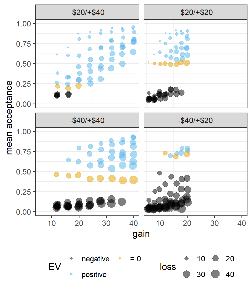

This call contains a few detailed specifications (e.g., nicer axes labels and better organised legends) typically only needed in a polished plot for a publication or presentation at a conference. The way to set these elements is therefore something that one can easily forget. One way to remember is by taking a look at the ggplot2 cheat sheet. Another way is by simply googling what you want to do. For example, I googled "ggplot2 legend two rows" to remember I needed to use guides() and the exact syntax. So, don't forget that google is your friend when it comes to R programming, especially for the tidyverse.

The plot shows the pattern across lotteries that we have seen before, and one that highly questions the original idea of loss aversion. It is clear that the relative attractiveness of symmetric lotteries differs considerably across conditions, so people do not evaluate the same magnitudes of losses and wins similarly across them.

4.8.3 By-Participant Plot

One important piece of information that the by-lottery plots do not show, is the variability in accepting the symmetric lotteries across participants. To visualise this, we need to plot the distribution of mean acceptability scores across participants for each condition separately. In particular, we are interested in these values for the three symmetric lotteries that are shared across all three conditions, the -$12/+$12, -$14/+$14, and -$16/+$16 lotteries.

To plot these values across participants, we first need to calculate the by-participant mean acceptability scores for the three symmetric lotteries. For this, we can use the filter introduced earlier and then group by both condition and subno.

part_sum <- ws1 %>%
  filter(loss == gain, loss %in% c(12, 16, 20)) %>% 
  group_by(condition, subno) %>% 
  summarise(mean_acc = mean(resp)) %>% 
  ungroup()
#> `summarise()` has grouped output by 'condition'. You can
#> override using the `.groups` argument.
part_sum
#> # A tibble: 781 × 3
#>   condition subno   mean_acc
#>   <fct>     <fct>      <dbl>
#> 1 -$20/+$40 e1a_109        0
#> 2 -$20/+$40 e1a_113        0
#> 3 -$20/+$40 e1a_125        0
#> 4 -$20/+$40 e1a_129        0
#> 5 -$20/+$40 e1a_13         0
#> 6 -$20/+$40 e1a_133        0
#> # ℹ 775 more rows

One problem we have when plotting this data is that there are only three shared symmetric lotteries, so we only have four distinct values for the mean acceptability scores.. Any individual participant can accept only 0, 1, 2 or 3 lotteries. Calculating the mean acceptability by dividing 0 to 3 by 3 gives four possible values:

0:3 / 3
#> [1] 0.0000000 0.3333333 0.6666667 1.0000000

## these are exactly the only values that occur in this data set:
sort(unique(part_sum$mean_acc))
#> [1] 0.0000000 0.3333333 0.6666667 1.0000000

In the code above, we used the : operator to create a sequence of integers (i.e., whole numbers) from 0 to 3. The same result would have been obtained by explicitly creating this vector, for example, using c(0, 1, 2, 3).

Plotting data like this with few unique values is a bit tricky. Our usual approaches -- alpha blending, jitter, bee swarm plots, or the like -- do not produce satisfactory results. The following code will produce all these plots and show the problem.

In this code, we also introduce another ggplot2 functionality. A plot created by ggplot2 is an R object itself. So far, we have printed the object which produces the plot in the plot pane. However, if we save the plot in an R object using <-, the plot is not shown in the plot pane. Instead, we can then use another function, such as plot_grid() from the cowplot package, to create one plot that consists of multiple individual plots. Note that you will have to install cowplot before running the code below (e.g., via install.packages("cowplot")).

## load packages required here:
library("cowplot")
#> 
#> Attaching package: 'cowplot'
#> The following object is masked from 'package:lubridate':
#> 
#>     stamp
library("ggbeeswarm")

p1 <- ggplot(part_sum, aes(x = condition, y = mean_acc)) +
  geom_point(alpha = 0.1) +
  stat_summary()
p2 <- ggplot(part_sum, aes(x = condition, y = mean_acc)) +
  geom_jitter(alpha = 0.1, width = 0.3, height = 0.1) +
  stat_summary()
## we set groupOnX = FALSE to avoid a warning otherwise
p3 <- ggplot(part_sum, aes(x = condition, y = mean_acc)) +
  geom_beeswarm(alpha = 0.1, groupOnX = TRUE, cex = 0.1) +
  stat_summary()
#> Warning: The `groupOnX` argument of `geom_beeswarm()` is deprecated
#> as of ggbeeswarm 0.7.1.
#> ℹ ggplot2 now handles this case automatically.
#> This warning is displayed once every 8 hours.
#> Call `lifecycle::last_lifecycle_warnings()` to see where
#> this warning was generated.
p4 <- ggplot(part_sum, aes(x = condition, y = mean_acc)) +
  geom_quasirandom(alpha = 0.1, groupOnX = TRUE) +
  stat_summary()
p5 <- ggplot(part_sum, aes(x = condition, y = mean_acc)) +
  geom_boxplot() +
  stat_summary()
p6 <- ggplot(part_sum, aes(x = condition, y = mean_acc)) +
  geom_violin(draw_quantiles = c(0, 0.25, 0.5, 0.75)) +
  stat_summary()
plot_grid(p1, p2, p3, p4, p5, p6, ncol = 2)
#> No summary function supplied, defaulting to
#> `mean_se()`
#> No summary function supplied, defaulting to `mean_se()`
#> No summary function supplied, defaulting to `mean_se()`
#> No summary function supplied, defaulting to `mean_se()`
#> No summary function supplied, defaulting to `mean_se()`
#> No summary function supplied, defaulting to `mean_se()`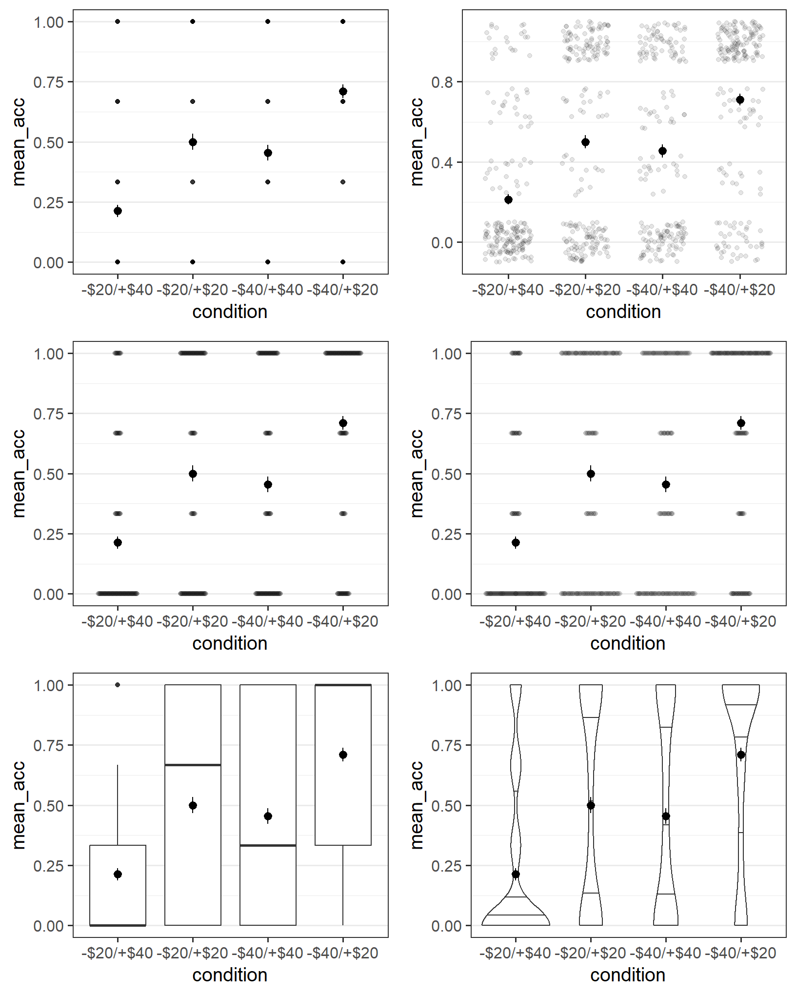

In my opinion, these six plots are all somewhat unsatisfactory. Perhaps the best one is the plot using jitter, but even here, the pattern in the data is not very clear.

An alternative for this particular situation is to not show all the individual data points, but the count of the data points that share one position. This can be achieved using geom_count. In the resulting plot, the size of the points will show how many points there are at each position.

ggplot(part_sum, aes(x = condition, y = mean_acc)) +
  geom_count(alpha = 0.2) +
  stat_summary()
#> No summary function supplied, defaulting to
#> `mean_se()`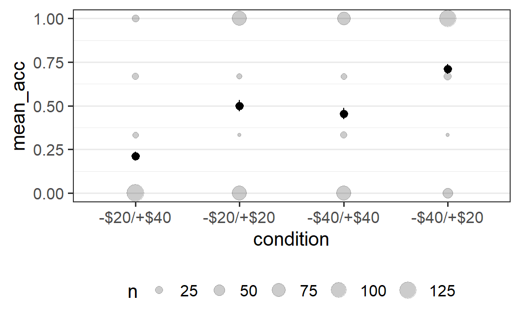

Instead of showing the count directly, we can also show the proportion of responses within each condition. As above, we can make this plot nicer by changing some labels. We can also adapt the grid lines in the background to be exactly at the 4 possible positions of the mean acceptabilities.

ggplot(part_sum, aes(x = condition, y = mean_acc)) +
  geom_count(aes(size = after_stat(prop)), alpha = 0.2) +
  stat_summary() +
  scale_y_continuous(breaks = c(0, 0.33, 0.67, 1)) +
  guides(size=guide_legend(title = "proportion")) +
  labs(y = "mean acceptance")
#> No summary function supplied, defaulting to
#> `mean_se()`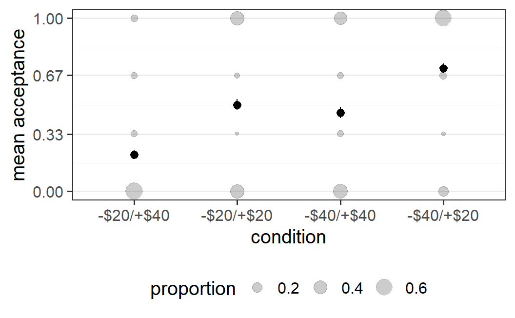

This plot shows that the distribution of individual mean acceptability scores is mostly bimodal. In all but the -$20/+$40 condition, the vast majority of participants either accepts all symmetric lotteries or rejects all of them. In the -$20/+$40 condition we only see one mode, which is when participants reject all symmetric lotteries. Taken together, this indicates that, overall, participants are quite consistent in their behaviour across different symmetric lotteries. If I reject or accept one symmetric lottery I am likely to make the same choice for another symmetric lottery. In other words, the amount of noise within participants is comparatively low whereas there is considerable noise across participants.

In addition, the plot clearly shows the main pattern of results. The original notion of loss aversion is that what matters for the acceptance rates of symmetric lotteries is the magnitude of the potential losses and gains. The present results clearly contradict this notion. In the -$20/+$40 condition, in which symmetric lotteries are unattractive, most participants reject them. In contrast, in the -$40/+$20 condition, in which symmetric lotteries are attractive, most participants accept them. In the two conditions in which the symmetric lotteries are neither particularly attractive nor unattractive, around half of the participants accept the symmetric lotteries and around half reject them.

Let's discuss a bit what I meant by"clearly shows" in the start of the paragraph above. The plot shows both the main results pattern as well as the variability in the data in such a way that this plot, in some sense, makes further statistical analysis not really necessary. Given the relatively large number of participants per condition (around 200), the fact that in one condition the vast majority never accepts a symmetric lottery, but in another condition the vast majority always accepts a symmetric lottery, means that there is a clear difference between conditions. Any reasonable statistical test must come to the same conclusion, otherwise we would begin to question the validity of the statistical test or look for some other problems with the data.

This means that a visual representation of the results can provide empirical evidence in addition to the statistical results. In fact, these two types of evidence -- figures derived from the results and statistical analyses derived from the results -- are complementary and should always be part of any communication of what you have found in an experiment. Without a figure, we cannot properly judge how much evidence the statistical result actually provides.

In the present case, in which the visual impression suggests a clear effect, some statisticians say the data pass the inter-ocular trauma test: The results hit you right between the eyes. If this is the case, our confidence that the data support an empirical hypothesis grows compared to a situation that only shows the outcome of a statistical analysis. If the statistical tests suggest an effect but the figures not so much, this is also an important outcome as it suggests the epistemic status of the empirical hypothesis is less clear. In any case, statistical analyses should always be accompanied by figures.

With this, we leave loss aversion and the study by Walasek and Stewart (2015) behind us. This example has shown rather extensively that finding evidence that appears to support our theoretical idea does not mean our theory is actually supported. Put more bluntly, it does not really look as if the original notion of loss aversion is tenable. Does this mean the rank-based account preferred by Walasek and Stewart (2015) is true? Not necessarily. What the data shows is that participants change their behaviour in a context-dependent manner. This is consistent with a rank-based account, but I am sure other accounts are possible as well. The larger point is that making strong inferences about great theoretical ideas is generally difficult.

4.9 Quiz

Note: The pull-down menu for selecting an answer turns green after selecting the correct answer.

Exercise 4.1 What data format does ggplot2 accept?

1. individual datapoints
2. data.frame / tibble
3. numerical vectors

Answer: 1 2 3

Exercise 4.2 What is the role of aes() function?

1. It tells R which data.frame we want to plot
2. It allows adding individual data points and lines to the plot
3. It is used to map variables in the data onto aesthetics

Answer: 1 2 3

Exercise 4.3 Which variable is typically plotted on the y-axis?

1. The independent variable
2. The dependent variable
3. The control variable

Answer: 1 2 3

Exercise 4.4 What does "over-plotting" refer to?

1. When at least two data points are at exactly the same position and cannot be visually differentiated
2. It means we created too many plots and need to restart R through the menu (Session - restart R)
3. It occurs when incorrect aesthetics have been used and ggplot2 cannot create a plot

Answer: 1 2 3

Exercise 4.5 What is "alpha blending"?

1. It is a synonym for "aesthetics" in ggplot2
2. A technique that creates the visual impression of semi-transparency
3. An argument to ggplot() indicating that we want to plot all points of the data

Answer: 1 2 3

Exercise 4.6 What does geom_jitter() do?

1. It introduces some random jitter for the plotted points
2. It allows a change of colour for some data points (i.e., colour is jittered)
3. It allows the combination of several plots into one bigger plot in a jittered manner

Answer: 1 2 3

Exercise 4.7 What is a "theme" in ggplot2?

1. It refers to a colour palette used for the plot
2. It is the title of a plot
3. The theme determines the overall look of a plot: e.g., font, font size, and background

Answer: 1 2 3

Exercise 4.8 What is a "faceted plot"?

1. A plot in which more than two variables are displayed
2. A plot in which data was originally over-plotted, but is not any more
3. A plot consisting of several sub-plots/panels

Answer: 1 2 3

Exercise 4.9 Which of the following does NOT show all the individual data points?

1. geom_boxplot()
2. geom_beeswarm()
3. geom_quasirandom()

Answer: 1 2 3

Exercise 4.10 What does 25% quantile mean?

1. It's the data point for which 25% of the data points are larger
2. It's the data point for which 25% of the data points are smaller
3. It's the data point for which 25% of the data points can be larger or smaller

Answer: 1 2 3

Exercise 4.11 Why are dynamite plots NOT useful?

1. They show only the mean
2. They do not show the distribution of the data or any data points
3. They do not contain legends and plot labels

Answer: 1 2 3

Exercise 4.12 What is the name of the function that adds the mean of the data to the plot?

1. mean()
2. geom_point()
3. stat_summary()

Answer: 1 2 3

Exercise 4.13 Which of these plots do NOT involve two or more variables?

1. histogram
2. box plot
3. bar graph

Answer: 1 2 3

Exercise 4.14 What does a uniform distribution look like?

1. It has one clear mode and is symmetric
2. It has at least two modes that have the same height
3. It does not have a clear mode

Answer: 1 2 3

Exercise 4.15 Consider you have data from an experiment with a dependent variable score and independent variable condition. What would be the aes() call to plot this data in the conventional way?

1. aes(condition = x, score = y)
2. aes(condition = y, score = x)
3. aes(x = condition, y = score)
4. aes(y = condition, x = score)

Answer: 1 2 3 4

Exercise 4.16 What is the appropriate way to handle outliers that are identified by a box-plot?

1. Outliers should be removed from the analysis as they can influence the results to a large degree.
2. Any real data point that is collected needs to be included in the analysis. Removing an outlier can be seen as an instance of data fabrication.
3. We should repeat the analysis with and without outlier, to see if the results are robust to the presence or absence of the outlier.

Answer: 1 2 3

4.10 ggplot2 Exercise: Earworms and Sleep

For this exercise, let's return to the study by Scullin, Gao, and Fillmore (2021) investigating the relationship between earworms and sleep quality. Let's quickly recap the study design and research question here. For more details see Section 3.10.

The study was a sleep lab experiment in which participants heard some music before going to sleep. In the lyrics condition, the songs were the original versions of pop songs with lyrics. In the instrumental condition, these were instrumental versions of the pop songs.

The researchers were interested in two research questions:

1. Does listening to the original version of a pop song (with lyrics) or an instrumental version of it affect whether or not participants develop earworms? This research question was based on previous results and the authors expected the instrumental version to induce more earworms than the lyrical versions.

To investigate this question, the researchers asked the participants whether they experienced earworms at various times during the experiment (i.e., while falling asleep, during the night, in the morning, or after getting ready to leave the sleep lab)

2. Does sleep quality differ between participants in the lyrical music condition and the instrumental music condition (in which participants are expected to have more earworms)?

To investigate this question, the researchers used polysomnography and measured various objective sleep parameters. Here, we are specifically looking at sleep efficiency and sleep time.

A version of the original data file made available by Scullin, Gao, and Fillmore (2021) can be downloaded from here. As before, I recommend you download it to the data folder in your working directory and then you can read in the data with the following code. It makes sense to restart R before doing that, so we also reload the tidyverse. Let's prepare the data set as discussed in the previous exercise and then take a look at it.

library("tidyverse")
library("cowplot")  ## for plot_grid()
library("ggbeeswarm") ## for bee swarm plot
theme_set(theme_bw(base_size = 15) + 
            theme(legend.position="bottom", 
                  panel.grid.major.x = element_blank()))
earworm <- read_csv("data/earworm_study.csv")
#> Rows: 48 Columns: 19
#> ── Column specification ────────────────────────────────────
#> Delimiter: ","
#> chr  (7): group, gender, raceethnicity, nativeenglishspe...
#> dbl (12): id, relaxed, sleepy, earworm_falling_asleep, e...
#> 
#> ℹ Use `spec()` to retrieve the full column specification for this data.
#> ℹ Specify the column types or set `show_col_types = FALSE` to quiet this message.
earworm <- earworm %>% 
  mutate(
    id = factor(id),
    group = factor(group, levels = c("Lyrics", "Instrumental"))
  )
glimpse(earworm)
#> Rows: 48
#> Columns: 19
#> $ id                     <fct> 102, 103, 104, 105, 106, 10…
#> $ group                  <fct> Lyrics, Lyrics, Instrumenta…
#> $ relaxed                <dbl> 37, 96, 62, 83, 68, 78, 60,…
#> $ sleepy                 <dbl> 49, 10, 44, 97, 42, 52, 41,…
#> $ earworm_falling_asleep <dbl> 0, 0, 0, 0, 0, 0, 0, 0, 0, …
#> $ earworm_night          <dbl> 0, 0, 0, 0, 0, 0, 0, 0, 0, …
#> $ earworm_morning        <dbl> 0, 0, 0, 0, 0, 0, 1, 0, 0, …
#> $ earworm_control        <dbl> 1, 1, 0, 0, 0, 0, 1, 0, 0, …
#> $ sleep_efficiency       <dbl> 90.0, 95.7, 89.8, 94.1, 98.…
#> $ sleep_time             <dbl> 487.6, 519.4, 472.1, 494.8,…
#> $ age                    <dbl> 19, 21, 19, 20, 27, 18, 22,…
#> $ gender                 <chr> "Female", "Female", "Female…
#> $ raceethnicity          <chr> "Caucasian", "Caucasian", "…
#> $ nativeenglishspeaker   <chr> "Yes", "Yes", "Yes", "Yes",…
#> $ bilingual              <chr> "No", "No", "No", "No", "No…
#> $ height_inches          <dbl> 66, 68, 64, 69, 53, 62, 76,…
#> $ weight_lbs             <dbl> 145, 183, 135, 155, 89, 120…
#> $ handedness             <chr> "R", "L", "R", "R", "R", "R…
#> $ classrank              <chr> "Sophomore", "Junior", "Fre…

In addition to the variables relevant to our research questions, the data contains a number of control variables (the original data file included even more). We can see a total of 19 variables:

• id: Participant identifier
• group: experimental condition with two values: "Lyrics" versus "Instrumental"
• relaxed: question asking participants how relaxed they felt on a scale from 0 (= not relaxed) to 100 (= very relaxed) after listening to the music.
• sleepy: question asking participants how sleepy they felt on a scale from 0 (= not sleepy) to 100 (= very sleepy) after listening to the music. The next 5 variables concerned whether or not the participants reported having an earworm at different times:
• earworm_falling_asleep: Had earworm while trying to fall asleep last night? 0 = No; 1 = Yes
• earworm_night: Had earworm while waking up during the night? 0 = No; 1 = Yes
• earworm_morning: Had earworm while waking up this morning? 0 = No; 1 = Yes
• earworm_control: Had earworm at the control time point (after getting ready to leave the lab)? 0 = No; 1 = Yes
• sleep_efficiency: a percentage score obtained from the polysomnography (0 = very low sleep efficiency and 100 = very high sleep efficiency)
• sleep_time: total sleep time in minutes

The remaining variables are demographic ones whose meaning should be evident, except, perhaps, for classrank. This uses US nomenclature for what year of four the student participant is in (Freshman = year 1, Sophomore = year 2, Junior = year 3, and Senior = year 4) plus some additional values for staff, post-graduate students and (presumably) one missing value ('-').

Exercise 4.17 Let's begin by taking a look at the distribution of sleep quality and sleep time, the two dependent variables for the second research question, using histograms. Ideally, combine the two histograms into one plot as shown previously using plot_grid(). Remember that one important part of making histograms is picking the appropriate bin width. What do the distributions look like?

Histograms are produced with geom_histogram(). To pick the correct bin width, just try out a few.

Let's start with a basic histogram without changing any setting to geom_histogram(). For this, we pass the earworm data to ggplot(), set x aesthetic to the variable we want to plot and then just combine both plots into one.

p1 <- ggplot(earworm, aes(x = sleep_efficiency)) +
  geom_histogram()
p2 <- ggplot(earworm, aes(x = sleep_time)) +
  geom_histogram()
plot_grid(p1, p2)
#> `stat_bin()` using `bins = 30`. Pick better value with
#> `binwidth`.
#> `stat_bin()` using `bins = 30`. Pick better value with
#> `binwidth`.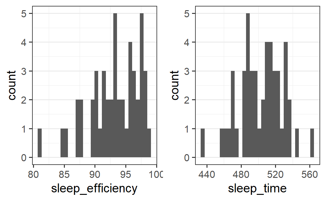

Both plots are a bit difficult to interpret as they are rather noisy, giving no clear visual impression. One possibility is that there are too many bins. Remember that we only have a total of 48 data points, so 30 bins means that there are few observations per bin.

Therefore, let's try to get a more informative visual impression by reducing the number of bins. Given the scale of the data we see here, let's start with a bin width of 2 for sleep efficiency and 10 for sleep time. Let's also set the boundary at 0 so the bins always begin at whole numbers.

p1 <- ggplot(earworm, aes(x = sleep_efficiency)) +
  geom_histogram(binwidth = 2, boundary = 0)
p2 <- ggplot(earworm, aes(x = sleep_time)) +
  geom_histogram(binwidth = 10, boundary = 0)
plot_grid(p1, p2)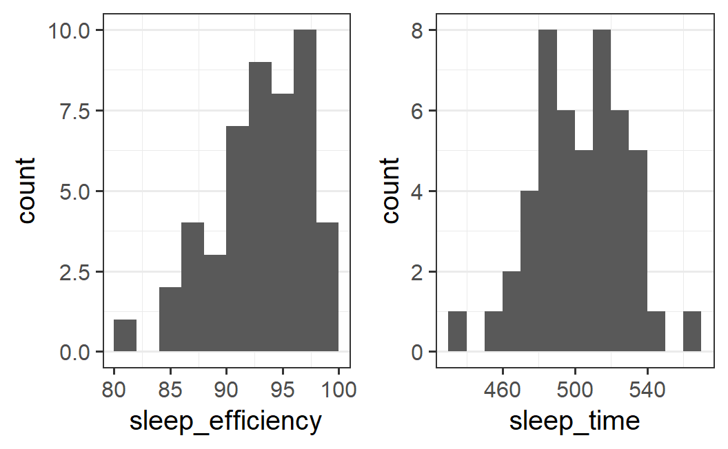

The resulting plots are much easier to interpret. The distribution of sleep efficiency scores is unimodal and asymmetric with a long tail on the left side (so-called left-skewed). The distribution of sleep times looks bi-modal but symmetric around the midpoint between the two modes.

To make sure this impression is not a fluke, let's make two more variants of each plot. In one, we halve the bin width, and in the other, we increase it by 50%.

## half bin width
p1 <- ggplot(earworm, aes(x = sleep_efficiency)) +
  geom_histogram(binwidth = 1, boundary = 0)
p2 <- ggplot(earworm, aes(x = sleep_time)) +
  geom_histogram(binwidth = 5, boundary = 0)
plot_grid(p1, p2)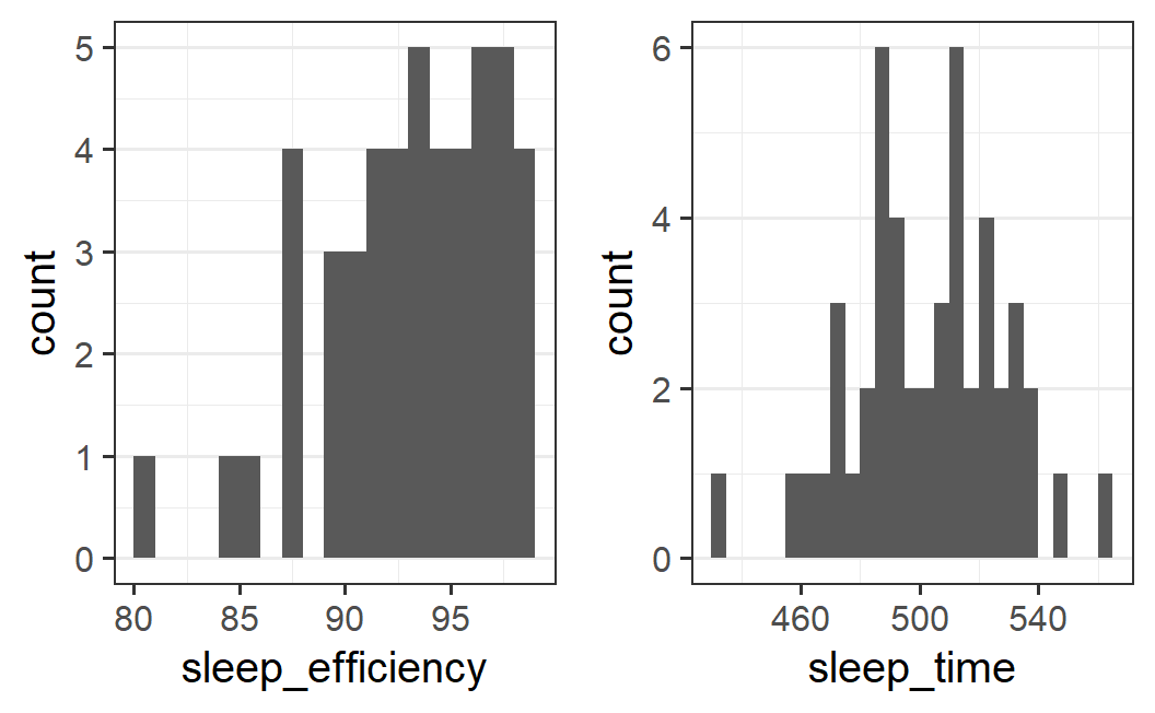

## 1.5 times bin width
p1 <- ggplot(earworm, aes(x = sleep_efficiency)) +
  geom_histogram(binwidth = 3, boundary = 100)
p2 <- ggplot(earworm, aes(x = sleep_time)) +
  geom_histogram(binwidth = 15, boundary = 0)
plot_grid(p1, p2)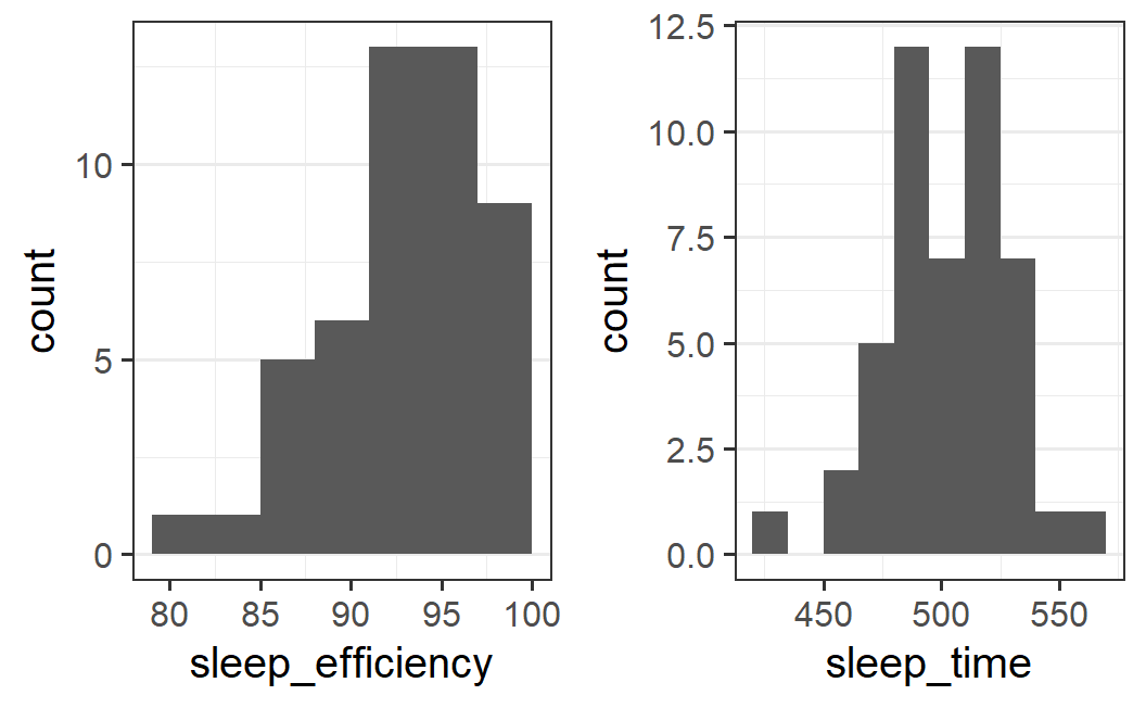

For sleep efficiency, the pattern is relatively stable. If we halve the bin width, the mode is less well defined. However, with 1.5 times the bin width, the pattern is very similar.

For sleep time, the pattern is essentially unchanged.

Let's make a final plot using the initial bin width, only a bit nicer. In particular, we harmonise the y-axis limits and use better x-axis labels.

p1 <- ggplot(earworm, aes(x = sleep_efficiency)) +
  geom_histogram(binwidth = 2, boundary = 0) +
  coord_cartesian(ylim = c(0, 11)) + 
  labs(x = "sleep efficiency")
p2 <- ggplot(earworm, aes(x = sleep_time)) +
  geom_histogram(binwidth = 10, boundary = 0) +
  coord_cartesian(ylim = c(0, 11)) + 
  labs(x = "sleep time (minutes)")
plot_grid(p1, p2)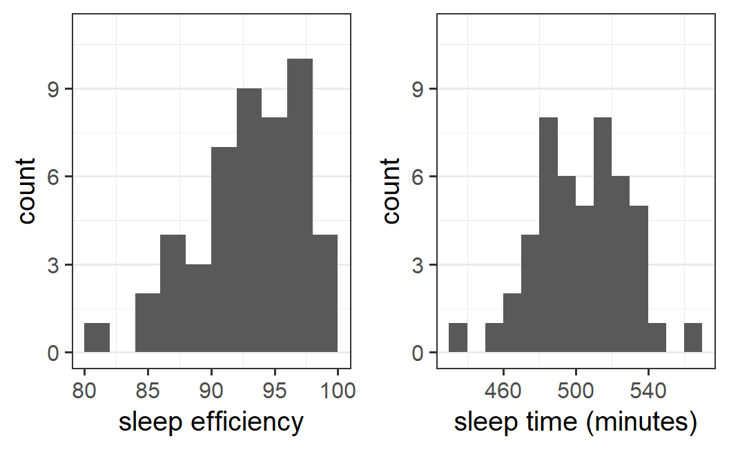

Exercise 4.18 The data contains two control variables, relaxed and sleepy, which are subjective judgements collected after participants listened to the music. As these variables are answers to relatively similar questions, we might suspect that participants provided similar responses. Make a plot of both control variables to see whether they are related.

Both control variables are continuous variables. Hence, you have to make a plot of two continuous variables. See Section 4.2 for details.

We can create this plot directly by passing the earworm data to ggplot() and mapping one of the variables to the x-axis and the other to the y-axis. Then we need to use geom_point() to see the data.

ggplot(earworm, aes(x = relaxed, y = sleepy)) +
  geom_point()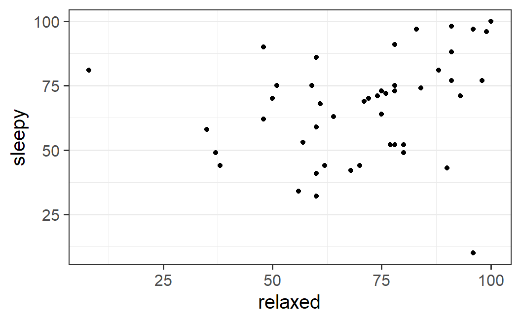 

This plot suggests that there seems to be a relationship, although it is certainly not strong. If the response to relaxed is large, the response to sleepy also appears to be large.

We can improve this plot to make this pattern somewhat clearer. Note that the data is on exactly the same scale for both variables, from 0 to 100. Thus, it makes sense to plot the data in a way that reflects this. In particular, we can make sure both axes show the full range of the scale, so that visually-judged distances mean the same for both axes. For this we can use coord_fixed() with ratio =1. Here. ratio refers to the aspect ratio of the plot, meaning its width divided by its height. A value of 1 therefore results in a plot that is square:

ggplot(earworm, aes(x = relaxed, y = sleepy)) +
  geom_point()  +
  coord_fixed(ratio = 1, xlim = c(0, 100), ylim = c(0, 100))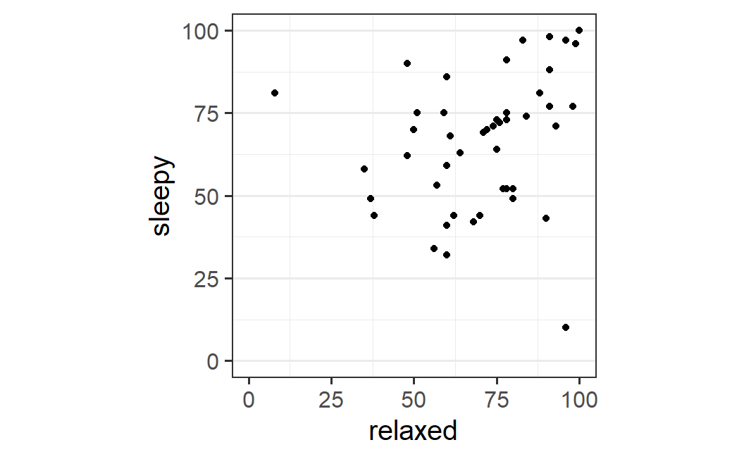

This plot makes it clearer that there seems to be a relationship, but that there are also two data points violating the general trend. In one case, sleepiness is large and relaxed is small. In the other, relaxed is large, but sleepiness is small.

Exercise 4.19 We might also be interested in whether the two control variables, relaxed and sleepy, show a relationship with the main dependent variable, sleep efficiency. As we have seen, these two variables also appear to be at least somewhat related. Therefore, we might also be interested in the relationship between a combined measure of these two control variables (the average of relaxed and sleepy) with sleep efficiency.

To check this, make three plots, one for each control variable plus one for the average of the two control variables. In each of these plots, one of the now three control variables is shown together with sleep efficiency. Are there obvious relationships of the control variables with sleep efficiency?

The control variables and sleep efficiency are continuous variables. So we have to plot two continuous variables in each plot. For more, see Section 4.2.

It also makes sense to first create the combined control variable, say control_combined before plotting it. For this, we can use mutate().

Let's begin by creating the combined control variable, control_combined using mutate.

earworm <- earworm %>% 
  mutate(control_combined = (relaxed + sleepy) / 2 )

Then, we can create one plot comparing each of the three control variables with sleep efficiency.

pe3_1 <- ggplot(earworm, aes(x = relaxed, y = sleep_efficiency)) +
  geom_point() 
pe3_2 <- ggplot(earworm, aes(x = sleepy, y = sleep_efficiency)) +
  geom_point() 
pe3_3 <- ggplot(earworm, aes(x = control_combined, y = sleep_efficiency)) +
  geom_point() 
plot_grid(pe3_1, pe3_2, pe3_3)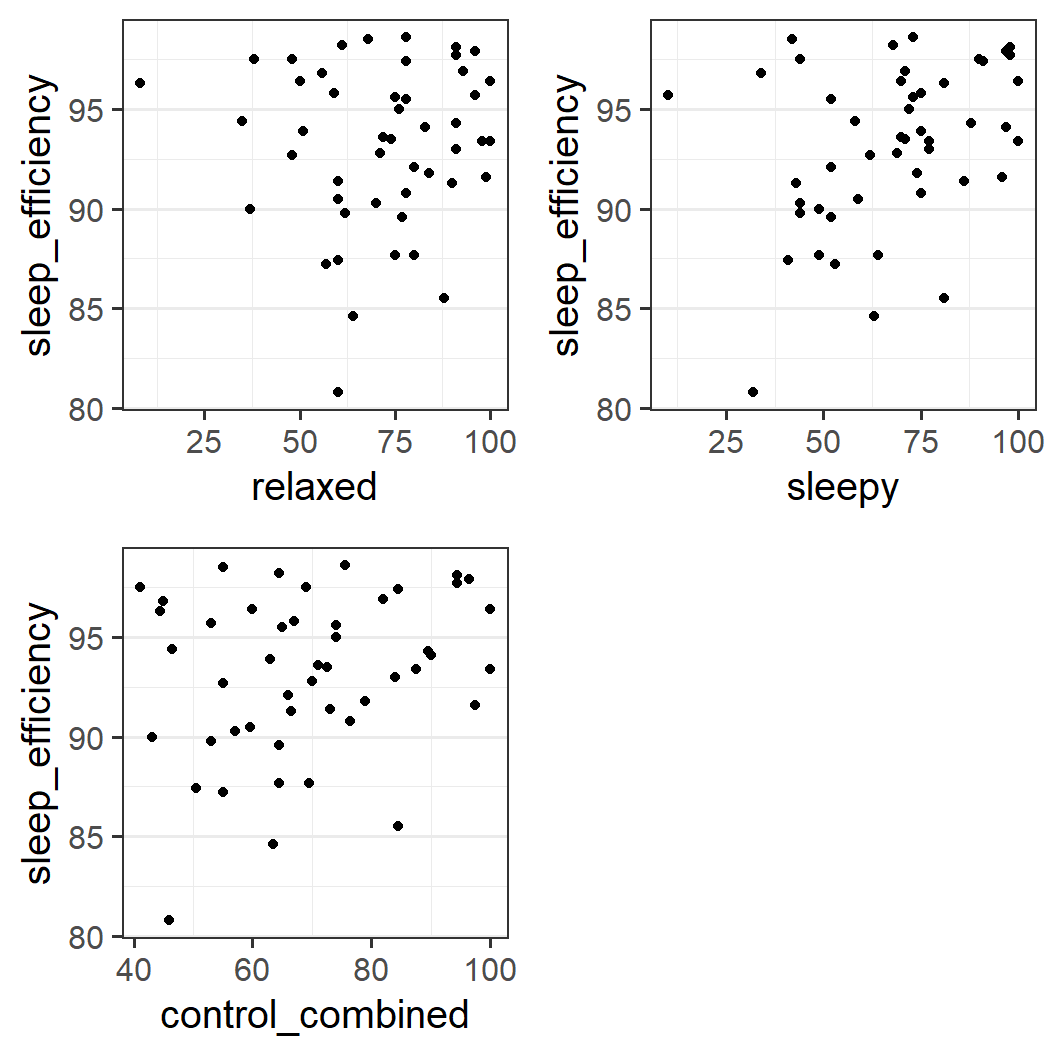

It is difficult to make a clear judgement here. For both relaxed and sleepy, there appear to be more data points in the top right of the plot than elsewhere. However, in both plots there is also one data point with a large sleep efficiency value that at the same time has the smallest value on the control variable. Note that these two unusual points are from different participants.

For sleepy however, there is also one data point with both small sleep efficiency and low sleepiness. For relaxed such a point is missing.

For the combined score, we also do not see a clear relationship. Whereas it looks like most data points are above the main diagonal (i.e., no data points in the lower right corner) there is not much more to say.

Exercise 4.20 Let's now take a look at research question (1): Does listening to the original version of a pop song (with lyrics) or an instrumental version of it affect whether or not participants develop earworms?

To do so, let's look at two different dependent variables we have created in the tidyverse exercise: any earworm at all (which should be 0 if the participant did not report any earworm and 1 otherwise) and proportion of earworms (which should be the sum of the three earworm dependent variables divided by 3). Then calculate whether group affects these two new dependent variables.

Note that we follow Scullin, Gao, and Fillmore (2021) and calculate these variables with only three of the earworm variables (i.e., all the earworm_... variables with the exception of earworm_control).

Make one plot for each of the two dependent variables in which the distribution of the variable across participants as well as the mean is shown, separately for each of the two experimental conditions.

Does the plot support the prediction that instrumental music leads to more earworms than lyrical music?

Now we have to make plots involving one categorical variable, experimental condition, and one continuous variable, the dependent variable. If this does not yet ring a bell, see Section 4.5.

We begin by creating the new variables. For this we can use the solution from the corresponding tidyverse exercise:

earworm <- earworm %>% 
  mutate(
    prop_earworm = (earworm_falling_asleep + earworm_night + 
                      earworm_morning) / 3
  ) %>% 
  mutate(any_earworm = if_else(prop_earworm == 0, 0, 1)) 

With this, we can start by making our plots beginning with prop_earworm. Note that prop_earworm has the same structure as the mean acceptance rate to the symmetric lotteries discussed in the example above. That means, there are only a few possible values, here four.

sort(unique(earworm$prop_earworm))
#> [1] 0.0000000 0.3333333 0.6666667 1.0000000

Hence, we can use essentially the same code as above and plot the count (or proportion) of the individual data points in the background. We only need to make sure to change the variables correctly.

ggplot(earworm, aes(x = group, y = prop_earworm)) +
  geom_count(aes(size = after_stat(prop)), alpha = 0.2) +
  stat_summary() +
  scale_y_continuous(breaks = c(0, 0.33, 0.67, 1)) +
  guides(size=guide_legend(title = "prop. participants")) +
  labs(y = "prop. earworms")
#> No summary function supplied, defaulting to
#> `mean_se()`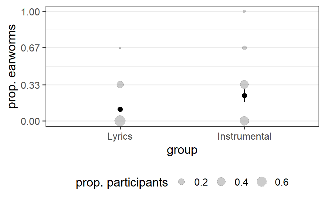

This plot provides some evidence for the hypothesis that instrumental songs induce earworms. In the 'lyrics' condition, the vast majority of participants report no earworms and only few report some. In contrast, in the 'instrumental' condition, participants are more likely to report earworms. Some even report having had earworms at each of the measured time points. Consequently, we also see a mean difference in the proportion of earworms here.

Let's now take a look at the second dependent variable, any_earworm. This variable can take on only two values, 0 or 1, per participant. Hence, we can use a very similar piece of code.

ggplot(earworm, aes(x = group, y = any_earworm)) +
  geom_count(aes(size = after_stat(prop)), alpha = 0.2) +
  stat_summary() +
  scale_y_continuous(breaks = c(0, 0.33, 0.67, 1)) +
  guides(size=guide_legend(title = "prop. participants")) +
  labs(y = "any earworm")
#> No summary function supplied, defaulting to
#> `mean_se()`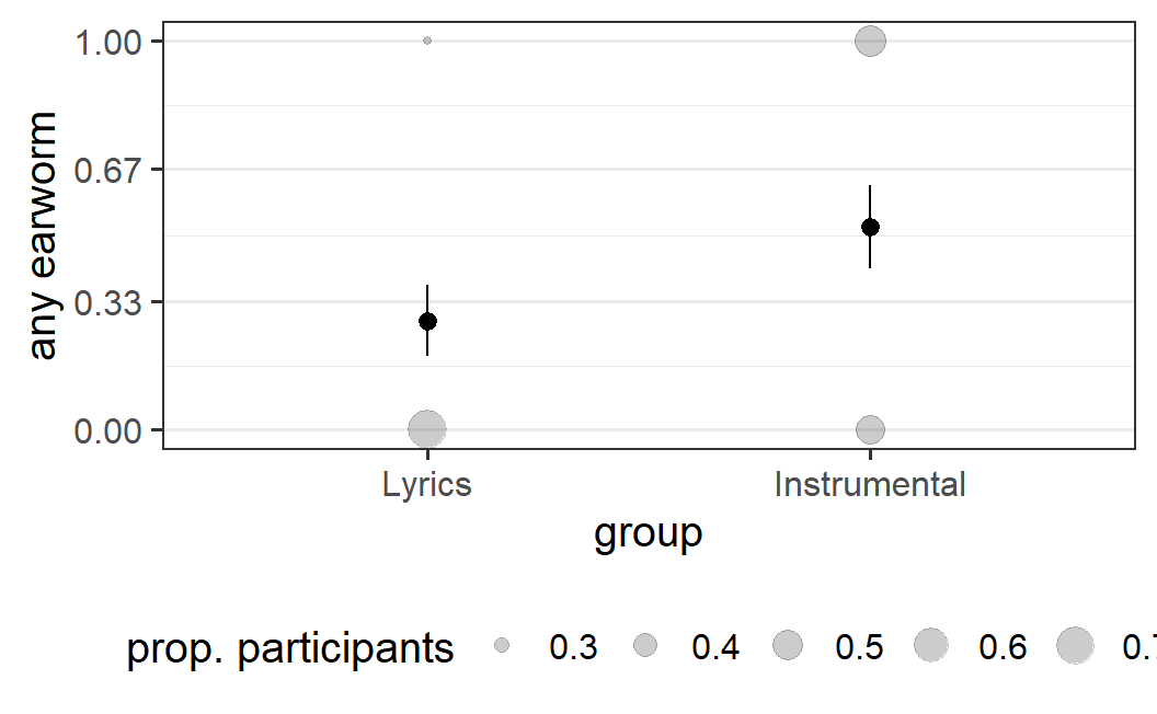

This provides a very similar picture as the 'any earworm' variable. For the 'lyrics' condition, the vast majority reports no earworms, whereas in the 'instrumental condition' the split is roughly 50-50. Of course, this similarity should not be too surprising. Both variables use the exact same information, only in slightly different ways.

In sum, the data supports the prediction that listening to instrumental music leads to more earworms than listening to lyrical music.

Exercise 4.21 Now that we have learned something about the relationship between different versions of pop songs and earworms, let's link this to the main point of interest of the study, sleep quality. More specifically, research question (2) is: Does sleep quality differ between participants in the lyrical music condition and the instrumental music condition, in which participants are expected to have more earworms?

Make one plot for each of the two dependent variables relevant to this research question, one for sleep efficiency and one for sleep time. As before, in each plot make sure that you show both the distribution of the variable across participants as well as the mean, separately for each of the two experimental conditions.

Does the plot support the hypothesis that the type of music heard before sleeping affects sleep quality?

We have to make a very similar plot as for the previous exercise. However, this time we probably want to show the individual data points somewhat differently.

For this exercise, we do not need to further manipulate the data as each participant has only one observation for both dependent variables. The most important question here is how to display the data in the background. Let's begin by using geom_beeswarm(),and make two plots, one for each dependent variable, and combine them into one figure.

pr2_1a <- ggplot(earworm, aes(x = group, y = sleep_efficiency)) +
  geom_beeswarm(alpha = 0.2) +
  stat_summary() 
pr2_2a <- ggplot(earworm, aes(x = group, y = sleep_time)) +
  geom_beeswarm(alpha = 0.2) +
  stat_summary() 
plot_grid(pr2_1a, pr2_2a)
#> No summary function supplied, defaulting to `mean_se()`
#> No summary function supplied, defaulting to `mean_se()`

This figure shows that for each of the two dependent variables, sleep quality is on average lower in the instrumental music group compared to the lyrical music group. When looking at the individual data points in the background, it looks like not many have the same value of the dependent variable, so the distribution of points is not very clear. Therefore, let's also try out using geom_quasirandom():

pr2_1b <- ggplot(earworm, aes(x = group, y = sleep_efficiency)) +
  geom_quasirandom(alpha = 0.2) +
  stat_summary() 
pr2_2b <- ggplot(earworm, aes(x = group, y = sleep_time)) +
  geom_quasirandom(alpha = 0.2) +
  stat_summary() 
plot_grid(pr2_1b, pr2_2b)
#> No summary function supplied, defaulting to `mean_se()`
#> No summary function supplied, defaulting to `mean_se()`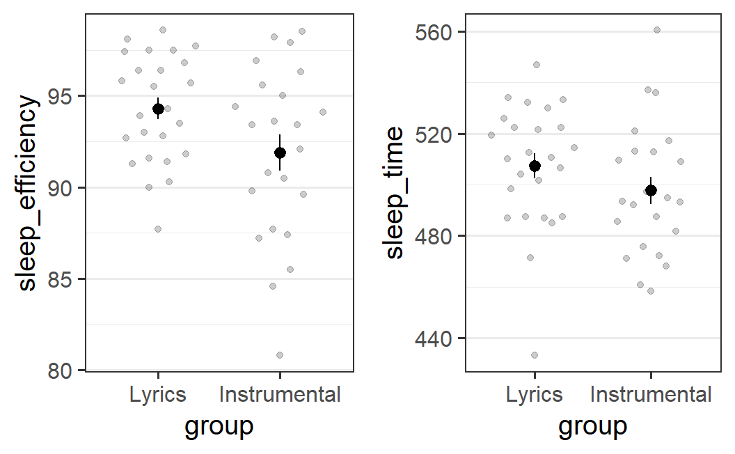

This plot shows more clearly that for sleep efficiency, there is a difference in the means that is also reflected in the distribution of individual points. For the instrumental condition, the distribution of points seems to have a bigger range, as well as being shifted downwards compared to the lyrical condition. This suggests that there might be an actual effect of the type of music listened to before sleep on sleep efficiency.

The pattern of results is not so clear for sleep time. Whereas there is also a difference in the means, the distributions look fairly similar. Furthermore, for each of the two groups there is one data point far away from the rest of the distribution (a potential "outlier") in opposite direction to the mean difference (i.e., a particularly low value for the lyrics group for which the mean is larger). Hence, whether the observed difference reflects a genuine difference is a lot less clear.

Speaking more generally, geom_quasirandom seems to provide the more interesting and easy to interpret data visualisation for this data set. It shows that there seems to be an effect of experimental condition on sleep efficiency, but the effect is less clear for sleep time.

Exercise 4.22 As a last exercise, make a plot that shows the distribution and means of sleep efficiency and sleep time conditional on whether or not participants had earworms during the night (i.e., at any time, excluding the control time point). Thus, in this analysis we ignore the experimental condition.

To perform the analysis, you need to begin with the same step as the corresponding analysis in the tidyverse exercises and then create one more set of plots:

1. Create a new factor, has_earworm, that is yes, whenever participants report at least once that they had an earworm for one of the three earworm dependent variables (i.e., within the experimental time frame, ignoring the control time).
2. Make a plot of sleep_efficiency and sleep_time as a function of has_earworm.
3. To ensure you do not forget to look into this, also calculate how many participants there are that do have versus do not have earworms.

What can you see? Do participants that report having an earworm sleep better than participants that do not do so, ignoring the experimental condition?

Take a look at the last tidyverse exercise to get going.

To create the new factor, has_earworm, we can transform any_earworm into a factor:

earworm <- earworm %>% 
  mutate(has_earworm = factor(
    any_earworm,
    levels = c(1, 0),
    labels = c("yes", "no")
  ))

We can then make the same plot as for the last analysis, but with a new independent variable.

pr3_1b <- ggplot(earworm, aes(x = has_earworm, y = sleep_efficiency)) +
  geom_quasirandom(alpha = 0.2) +
  stat_summary() 
pr3_2b <- ggplot(earworm, aes(x = has_earworm, y = sleep_time)) +
  geom_quasirandom(alpha = 0.2) +
  stat_summary() 
plot_grid(pr3_1b, pr3_2b)
#> No summary function supplied, defaulting to `mean_se()`
#> No summary function supplied, defaulting to `mean_se()`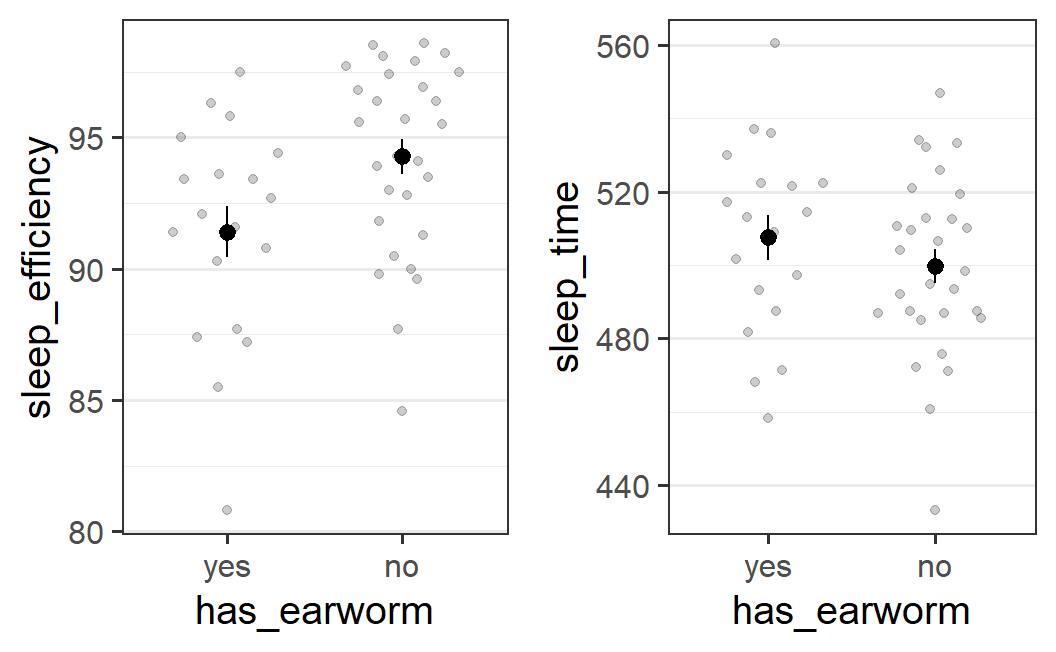

This plot suggests that sleep efficiency is lower if one reports at least one earworm during the night compared to when not. Interestingly, participants that report no earworms show a unimodal distribution with a mode that is larger than all but one sleep efficiency score for participants that do report earworms. However, as both distributions have a relatively long tail towards lower scores, the difference in means is not huge.

For sleep time, the difference is in the opposite direction and noticeably smaller.

The plot also shows that there are fewer participants that report an earworm than those that do not. Let's take a look again how large both groups are:

earworm %>% 
  group_by(has_earworm) %>% 
  summarise(n = n()) %>% ## calculate N
  mutate(prop = n/sum(n)) ## transform N into %
#> # A tibble: 2 × 3
#>   has_earworm     n  prop
#>   <fct>       <int> <dbl>
#> 1 yes            19 0.396
#> 2 no             29 0.604

This shows that around 40% of participants report an earworm, indicating that the imbalance is not very large.