Standard Approach for One IV: Quiz and Exercises

6.7 Quiz

Note: The pull-down menu for selecting an answer turns green after selecting the correct answer.

Exercise 6.1 What is NOT true about the sample?

The sample are a subset of the population
The sample encompasses all individual that could in principle take part in the study
The sample are the actual participants of a study

Answer:

Exercise 6.2 In a typical experiment with the participants being mostly undergraduate students, what is the population?

All undergraduate students (including past and future undergraduate students)
All humans (i.e., the human population in general)
Undergraduate students from the university where the experiment was done

Answer:

Exercise 6.3 What is the goal of "descriptive statistics"?

Description of data patterns in the population
Description of data patterns in the sample
Generalising from sample to population

Answer:

Exercise 6.4 What is the goal of "inferential statistics"?

Description of data patterns in the population
Description of data patterns in the sample
Generalising from sample to population

Answer:

Exercise 6.5 What does "NHST" stand for?

Non-hypothesis significance table
New hypothesis significant theory
Null hypothesis significance testing

Answer:

Exercise 6.6 What is a principle of the NHST approach of inferential statistics?

In the population, there either is no difference in the condition means or there is a difference in the condition means
If there is no difference in condition means in the sample, there is also no difference in the condition means in the population
The approach is valid only when the condition means in the population are significantly different

Answer:

Exercise 6.7 What is NOT true about the NHST?

NHST allows to prove if there is a mean difference in population
NHST checks the compatibility of the data with the null hypothesis
All inferences based on the NHST are probabilistic

Answer:

Exercise 6.8 What is NOT a part of the basic statistical model?

DV
IV
Intercept
Median
Residuals

Answer:

Exercise 6.9 What are residuals?

Conditions means
Differences between observed predicted values
The sum of the IV-effect and intercept

Answer:

Exercise 6.10 What is NOT an ANOVA?

A statistical model that solely includes factors as IVs
Analysis of variance
A mandatory part of the basic statistical model

Answer:

Exercise 6.11 What is the \(p\)-value?

The probability that the null hypothesis is true (and therefore also the probability that our research question is false)
The probability of observing an effect at least as extreme as observed, assuming that the null hypothesis is true
The probability that the null hypothesis is false

Answer:

Exercise 6.12 What does it mean if \(p < .05\)?

The result is significant and we reject the null hypothesis
The result is not significant and we do not reject the null hypothesis
The null hypothesis is extremely unlikely and therefore probably false

Answer:

Exercise 6.13 How can you interpret the following statistical results: \(F(1, 38) = 0.54\), \(p = .002\)?

Because \(p < .05\), the result is significant and we reject the null hypothesis
Because \(p < .05\), our research question is supported by the data
Because \(p < .05\) and \(F < 1\), something must be wrong with the results

Answer:

Exercise 6.14 Imagine you run a direct replication of a previous study that found a particular significant result. What does it mean if the replication study is successful (i.e., also finds a significant results that is very similar to the previous result)?

A successful replication indicates that the theory of the researchers is probably true
A successful replication indicates that the original researchers did not make an error in their study
A successful replication indicates that the original result was probably not only due to chance

Answer:

Exercise 6.15 Imagine you run a direct replication of a previous study that found a particular significant result. What does it mean if the replication study fails (i.e., does not find a significant results that is very similar to the previous result)?

The original results must have been a false positive result
It reduces the evidence provided by original result
The replication results must be a false negative result

Answer:

6.8 Exercise: Earworms and Sleep

For this exercise, let's once again return to the study by Scullin, Gao, and Fillmore (2021) investigating the relationship between earworms and sleep quality. Let's quickly recap the study design and research question here. For more details see Section 3.10.

The study was a sleep lab experiment in which participants heard some music before going to sleep. In the lyrics condition, the songs were the original versions of pop songs with lyrics. In the instrumental condition, these were instrumental versions of the pop songs.

The researchers were interested in two research questions:

Does listening to the original version of a pop song (with lyrics) or an instrumental version of it affect whether or not participants develop earworms? This research question was based on previous results and the authors expected the instrumental version to induce more earworms than the lyrical versions.

To investigate this question, the researchers asked the participants whether they experienced earworms at various times during the experiment (i.e., while falling asleep, during the night, in the morning, or after getting ready to leave the sleep lab).

Does sleep quality differ between participants in the lyrical music condition and the instrumental music condition (in which participants are expected to have more earworms)?

To investigate this question, the researchers used polysomnography and measured various objective sleep parameters. Here, we are specifically looking at sleep efficiency and sleep time.

A version of the original data file made available by Scullin, Gao, and Fillmore (2021) can be downloaded from here. As before, I recommend you download it to the data folder in your working directory and then you can read in the data with the following code. It makes sense to restart R before doing that.

We then load the packages we need for this exercise, the tidyverse, afex, and emmeans. Let's prepare the data set as discussed in the previous exercise and then take a look at it.

library("afex")
library("emmeans")
library("tidyverse")
theme_set(theme_bw(base_size = 15) + 
            theme(legend.position="bottom", 
                  panel.grid.major.x = element_blank()))
earworm <- read_csv("data/earworm_study.csv")
earworm <- earworm %>% 
  mutate(
    id = factor(id),
    group = factor(group, levels = c("Lyrics", "Instrumental"))
  )
glimpse(earworm)
#> Rows: 48
#> Columns: 19
#> $ id                     <fct> 102, 103, 104, 105, 106, 10…
#> $ group                  <fct> Lyrics, Lyrics, Instrumenta…
#> $ relaxed                <dbl> 37, 96, 62, 83, 68, 78, 60,…
#> $ sleepy                 <dbl> 49, 10, 44, 97, 42, 52, 41,…
#> $ earworm_falling_asleep <dbl> 0, 0, 0, 0, 0, 0, 0, 0, 0, …
#> $ earworm_night          <dbl> 0, 0, 0, 0, 0, 0, 0, 0, 0, …
#> $ earworm_morning        <dbl> 0, 0, 0, 0, 0, 0, 1, 0, 0, …
#> $ earworm_control        <dbl> 1, 1, 0, 0, 0, 0, 1, 0, 0, …
#> $ sleep_efficiency       <dbl> 90.0, 95.7, 89.8, 94.1, 98.…
#> $ sleep_time             <dbl> 487.6, 519.4, 472.1, 494.8,…
#> $ age                    <dbl> 19, 21, 19, 20, 27, 18, 22,…
#> $ gender                 <chr> "Female", "Female", "Female…
#> $ raceethnicity          <chr> "Caucasian", "Caucasian", "…
#> $ nativeenglishspeaker   <chr> "Yes", "Yes", "Yes", "Yes",…
#> $ bilingual              <chr> "No", "No", "No", "No", "No…
#> $ height_inches          <dbl> 66, 68, 64, 69, 53, 62, 76,…
#> $ weight_lbs             <dbl> 145, 183, 135, 155, 89, 120…
#> $ handedness             <chr> "R", "L", "R", "R", "R", "R…
#> $ classrank              <chr> "Sophomore", "Junior", "Fre…

In addition to the variables relevant to our research questions, the data contains a number of control variables (the original data file included even more). We can see a total of 19 variables:

id: Participant identifier
group: experimental condition with two values: "Lyrics" versus "Instrumental"
relaxed: question asking participants how relaxed they felt on a scale from 0 (= not relaxed) to 100 (= very relaxed) after listening to the music.
sleepy: question asking participants how sleepy they felt on a scale from 0 (= not sleepy) to 100 (= very sleepy) after listening to the music. The next 5 variables concerned whether or not the participants reported having an earworm at different times:
earworm_falling_asleep: Had earworm while trying to fall asleep last night? 0 = No; 1 = Yes
earworm_night: Had earworm while waking up during the night? 0 = No; 1 = Yes
earworm_morning: Had earworm while waking up this morning? 0 = No; 1 = Yes
earworm_control: Had earworm at the control time point (after getting ready to leave the lab)? 0 = No; 1 = Yes
sleep_efficiency: a percentage score obtained from the polysomnography (0 = very low sleep efficiency and 100 = very high sleep efficiency)
sleep_time: total sleep time in minutes

The remaining variables are demographic ones whose meaning should be evident, except, perhaps, for classrank. This uses US nomenclature for what year of four the student participant is in (Freshman = year 1, Sophomore = year 2, Junior = year 3, and Senior = year 4) plus some additional values for staff, post-graduate students and (presumably) one missing value ('-').

Exercise 6.16 In the previous exercises, we we have already investigated the data rather comprehensively. Consequently, let's immediately jump in and analyse research question 1 using inferential statistics (i.e., an ANOVA).

Does the provide support for the hypothesis that the type of music listened to before going to bed affects the development of earworms?

To answer this question it is important to make a decision on what "development of earworms" means. In the previous exercises we look at least at two different interpretations: the proportion of time points for which participants reported having an earworm or did participants get any earworm during the night.

What do the result mean for the research question?

To analyse this research question, we first need to create a new dependent variable (DV) which tells us whether or not participants developed earworms during the night. We can then analyse this DV using aov_car().

To analyse this research question, we first need to create new dependent variables (DV) which tells us whether or not participants developed earworms during the night. For this, we can copy and paste a solution from a previous exercise that creates two variants of this DV, the proportion of time points for which participants reported having an earworm, prop_earworm, and a binary variable indicating whether participants got any earworm during the night, any_earworm.

earworm <- earworm %>% 
  mutate(
    prop_earworm = (earworm_falling_asleep + earworm_night + 
                      earworm_morning) / 3
  ) %>% 
  mutate(any_earworm = if_else(prop_earworm == 0, 0, 1))

With this new DVs we can use aov_car to see whether the type of music has a significant effect on the creation of earworms. Let's begin with prop_earworm. The formula has this as the DV and the experimental condition, group, as IV. We also need to pass the participant identifier column id in the Error() term.

res_1a <- aov_car(prop_earworm ~ group + Error(id), earworm)
#> Contrasts set to contr.sum for the following variables: group
res_1a
#> Anova Table (Type 3 tests)
#> 
#> Response: prop_earworm
#>   Effect    df  MSE      F  ges p.value
#> 1  group 1, 46 0.05 3.49 + .070    .068
#> ---
#> Signif. codes:  
#> 0 '***' 0.001 '**' 0.01 '*' 0.05 '+' 0.1 ' ' 1

The ANOVA table shows a non-significant effect of music type on the proportion of time points during which an earworm is reported.

We then also look at the second DV, any_earworm.

res_1b <- aov_car(any_earworm ~ group + Error(id), earworm)
#> Contrasts set to contr.sum for the following variables: group
res_1b
#> Anova Table (Type 3 tests)
#> 
#> Response: any_earworm
#>   Effect    df  MSE      F  ges p.value
#> 1  group 1, 46 0.23 2.99 + .061    .091
#> ---
#> Signif. codes:  
#> 0 '***' 0.001 '**' 0.01 '*' 0.05 '+' 0.1 ' ' 1

The ANOVA table, also reveals a non-significant result.

Before summarising the result, let's take a look at the estimated marginal means whether they are in line with the expectations:

emmeans(res_1a, "group")
#>  group        emmean     SE df lower.CL upper.CL
#>  Lyrics        0.107 0.0464 46   0.0132    0.200
#>  Instrumental  0.232 0.0484 46   0.1345    0.329
#> 
#> Confidence level used: 0.95
emmeans(res_1b, "group")
#>  group        emmean     SE df lower.CL upper.CL
#>  Lyrics        0.280 0.0968 46   0.0851    0.475
#>  Instrumental  0.522 0.1009 46   0.3186    0.725
#> 
#> Confidence level used: 0.95

This shows that in the instrumental condition, participants apear to be more likely to develop earworms.

Overall answer: Descriptively the results suggest that participants that listen to instrumental compared to lyrical music are more likely to report any earworm during the night (0.52 compared to 0.28). At the same time, participants in the instrumental condition report earworms at more time points during the nights than participants in the lyrical condition (0.23 compred to 0.11). However, these difference do not reach significance with an ANOVA with experimental condition as factor, neither for any earworm, F(1, 46) = 2.99, p = .091, nor for the proportion of time points for which earworms are reported, F(1, 46) = 3.49, p = .068.

Exercise 6.17 Analyse the second research question using NHST and an ANOVA: Does sleep quality differ between participants in the lyrical music condition and the instrumental music condition?

As the measure of sleep quality focus on sleep efficiency. But also check if the same pattern is observed for total time slept. Also make a result plot for each of the two measures of sleep quality and combine them into into one figure.

Then write a brief summary of the results.

For the analysis we can again use aov_car(). For plotting we can use afex_plot() and combine the plots with cowplot::plot_grid().

The data is already in the correct format for this task. Thus, we can immediately start with the analysis of the sleep efficiency:

res_2a <- aov_car(sleep_efficiency ~ group + Error(id), earworm)
#> Contrasts set to contr.sum for the following variables: group
res_2a
#> Anova Table (Type 3 tests)
#> 
#> Response: sleep_efficiency
#>   Effect    df   MSE      F  ges p.value
#> 1  group 1, 46 15.38 4.58 * .091    .038
#> ---
#> Signif. codes:  
#> 0 '***' 0.001 '**' 0.01 '*' 0.05 '+' 0.1 ' ' 1

The ANOVA table shows a significant effect of music condition. Let's take a look at sleep time as well:

res_2b <- aov_car(sleep_time ~ group + Error(id), earworm)
#> Contrasts set to contr.sum for the following variables: group
res_2b
#> Anova Table (Type 3 tests)
#> 
#> Response: sleep_time
#>   Effect    df    MSE    F  ges p.value
#> 1  group 1, 46 634.72 1.77 .037    .190
#> ---
#> Signif. codes:  
#> 0 '***' 0.001 '**' 0.01 '*' 0.05 '+' 0.1 ' ' 1

For sleep time we do not see a significant effect.

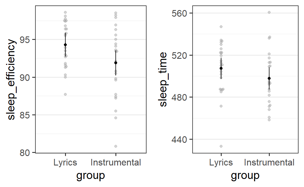
Let's create two results plot using afex_plot and combine them into one:

p1 <- afex_plot(res_2a, "group")
p2 <- afex_plot(res_2b, "group")
cowplot::plot_grid(p1, p2)

This shows that in the instrumental condition, participants appear to be more likely to develop earworms.

Summary: As shown in the figure, both sleep efficiency and sleep time is higher in the lyrics compared to the instrumental condition. Separate ANOVA analysis of these two dependent variables with experimental condition as factor (with levels lyrics vs. instrumental) reveals that this difference is significant for sleep efficiency, F(1, 46) = 4.58, p = .038, but nor for sleep time, F(1, 46) = 1.77, p = .190.

Exercise 6.18 The actual research question of the researchers is whether earworms reduce sleep quality or not. However, because it is unclear how earworms emerge, the researchers use the manipulation of the type of music listened to before going to bed to induce more earworms in the instrumental condition compared to the lyrical condition. In some sense, this is an indirect test of the actual research question.

A more direct test of the actual research question is to compare the sleep quality of participants that report earworms at any point during the night with the sleep quality of participants that do not report any earworms. Your task is to perform this more direct test statistically. What do the results show? How can we interpret them?

The R syntax is very similar to the answer of the previous two exercises and can reuse some of the variable created there. The question how to interpret the results requires you to think about what kind of variable the independent variable of the analysis is.

To test the research question if the sleep quality differs between participants that report or do not report earworms, we need to have a factor in our data that indicates whether a participant reported an earworm. The any_earworm variable crwated in a previous exercise contains this information, but is not a factor. Therefore, we transform it into a factor, has_earworm:

earworm <- earworm %>% 
  mutate(has_earworm = factor(any_earworm, 
                              levels = c(1, 0), 
                              labels = c("yes", "no")))

Then we can calculate the two ANOVAs for the two sleep quality measures. First for sleep efficiency:

res_3a <- aov_car(sleep_efficiency ~ has_earworm + Error(id), earworm)
#> Contrasts set to contr.sum for the following variables: has_earworm
res_3a
#> Anova Table (Type 3 tests)
#> 
#> Response: sleep_efficiency
#>        Effect    df   MSE      F  ges p.value
#> 1 has_earworm 1, 46 14.86 6.33 * .121    .015
#> ---
#> Signif. codes:  
#> 0 '***' 0.001 '**' 0.01 '*' 0.05 '+' 0.1 ' ' 1

As above, the ANOVA shows a significant effect. Let's run the same analysis for sleep time.

res_3b <- aov_car(sleep_time ~ has_earworm + Error(id), earworm)
#> Contrasts set to contr.sum for the following variables: has_earworm
res_3b
#> Anova Table (Type 3 tests)
#> 
#> Response: sleep_time
#>        Effect    df    MSE    F  ges p.value
#> 1 has_earworm 1, 46 643.60 1.11 .024    .298
#> ---
#> Signif. codes:  
#> 0 '***' 0.001 '**' 0.01 '*' 0.05 '+' 0.1 ' ' 1

As above, the ANOVA does not show a significant effect.

Let's also plot the two results:

p1 <- afex_plot(res_3a, "has_earworm")
p2 <- afex_plot(res_3b, "has_earworm")
cowplot::plot_grid(p1, p2)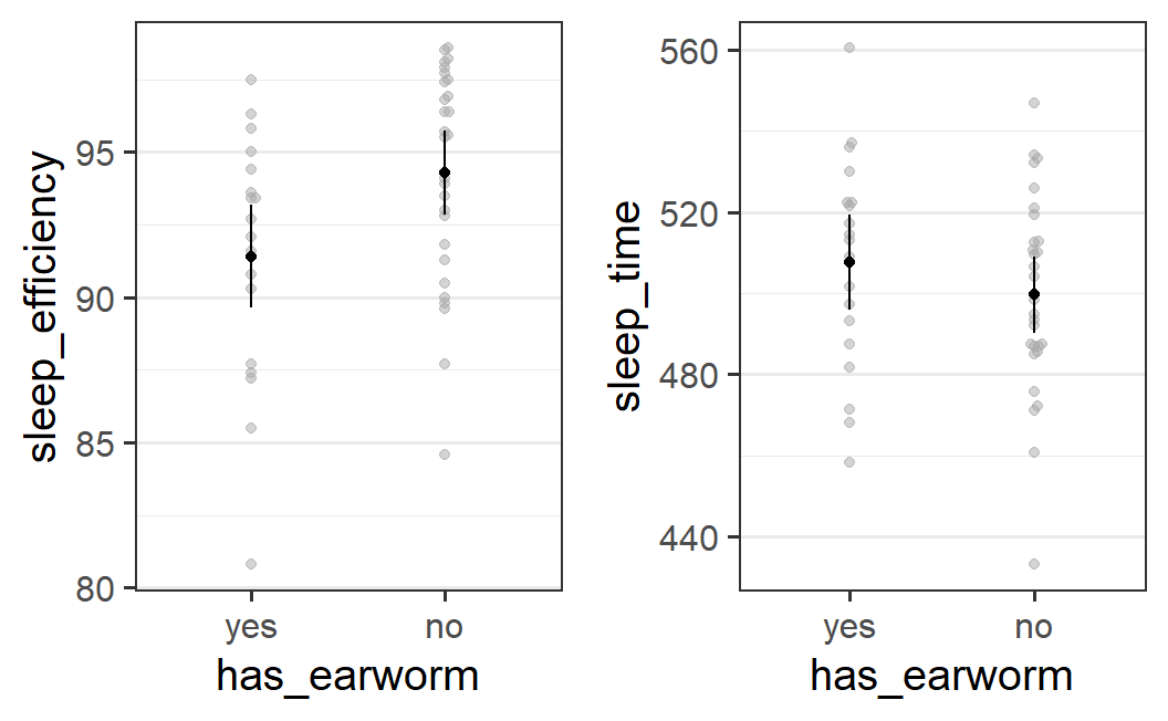

The plot reveals an interesting pattern. For sleep efficiency the results are in line with the results for the experimental manipulation. Having an earworm appears to reduce the sleep quality, F(1, 46) = 6.33, p = .015 (as does listening to instrumental music). However, for sleep time the results are not only not significant, F(1, 46) = 1.11, p = .298, the results are also descriptively not in line with the results from the experimental manipulation. Whereas for the type of music, participants in the instrumental condition appeared to sleep slightly less, participants that report an earworm appear to sleep slightly longer. Taken together this shows that time slept does not to be affected by either the experimental manipulation nor whether participants report an earworm.

Overall, we have now three different pieces of evidence: The instrumental compared to the lyrical conditions leads to somewhat more earworms (although this effect is not statistically significant) and also to worse sleep quality. Furthermore, participants that report earworms have a worse sleep quality than participants that report no earworms. Does this indicate that earworms are necessarily causally responsible for the worse sleep quality? Unfortunately we cannot conclude that. The problem is that we did not directly manipulate the presence of earworms, we only measured (or observed) whether participants have an earworm. Thus, we cannot rule out that there is another variable at play that is causally responsible for worse sleep quality and also related to the presence of earworms.

For example, we could imagine that the absence of language when listening to instrumental compared to lyrical music puts participants in a more creative mindset. Then, being in a creative mindset could both lead to worse sleep quality (because the mind is "creative" and therefore active) and also more earworms. Furthermore, more creative people would also report more earworms and sleep worse which would also explain the last result. This explanation is not particularly likely, because it is made up on the spot (i.e., I have no idea if there is a such thing as a "creative mindeset"). Nevertheless, it is able to explain all pieces of evidence discussed here without the necessity that earworms are causally resonsible for anything, they are just an epiphenomenon. Whenever a variable is not manipulated directly, such as earworms in the present study, we cannot easily make causal inferences as we can always come up with at least somewhat plausible alternative explanations.

6 Case Study: More Results from Note Taking Studies

References