3 Short Introduction to R and the tidyverse

The previous two chapters have provided the theoretical and conceptual background we need for performing a statistical analysis. In this chapter we switch focus to the practical side and introduce the basics of the tool that we will use to perform a statistical analysis in practice, the statistical programming language R.

As we have discussed in the previous chapters, the value of a scientific theory or hypotheses depends ultimately on the evidence that supports it. This evidence comes in the form of data. Thus, to be able to judge the strength of the evidence provided by the data, a central task in the research practice is to analyse and then interpret data. R is the tool that we will use for this task. It is one of the most comprehensive and popular tools for all aspects of data analysis.

3.1 What is R?

R is a comprehensive tool that enables the skilled user to perform all steps or tasks of a data analysis with it. For example, with R we can:

• Prepare data for analysis: read data that comes in pretty much any format, manipulate and wrangle data.
• Explore data using summary statistics and graphical summaries: exploratory data analysis, descriptive statistics, and data visualisation
• Perform statistical analysis of the data: inferential statistics
• Communicate the results: publication-ready results graphics, research reports that combine narrative text and statistical results
• And much more such as: data simulations and advanced statistical methods, machine learning, interactive data visualisations, websites, books (such as the present one)

On top of this incredible list of things that can be done with R, R is free software (sometimes also known as open source software). This means, not only is R completely free to download, install, and use, you are also free to inspect its source code or make changes to it (as long as you do not make your version of R un-free).

Given the flexibility of all the things you can do with R, it is not completely surprising that it requires some effort to get started with R. Especially if R is your first real experience of learning a programming language.

The important thing to know for any new R user is that the beginning is hard for almost everyone (including the present author), but using R gets a lot easier and smoother after some time and effort dedicated to learning the basics. The most important message is to hang in there and keep on trying. In all likelihood, there will be at least some rather frustrating situations in your first weeks of interacting with R, but it will get better. I have taught R to many users with a great variety of backgrounds and experiences and many of them have struggled in some way in the beginning. But for anyone who kept up their hopes and continued to put in the time and effort, their struggles were not in vain. You can learn R if you just believe in yourself and do not give up. Be assured I believe in you. Learning R is such an incredibly powerful skill that will surely have a positive effect on whatever comes later in your life, be it a career in Academia (i.e., at a university) or in "the real world" (as we academics like to call everything that is not a university job).

3.2 Getting Started with R

With this somewhat scary introduction out of the way, the next important question is probably how do you get going with R? Providing a comprehensive answer to this question is beyond the scope of the present work. Instead, we will point you to some freely available resources that we expect you to go through before continuing with the rest of the chapter so you get up to speed with R first. We begin with a list of minimum requirements you have to work through on your own before continuing. These will probably take some time, but must be done. After that, we provide links to some additional resources that you can also take a look at, either now or at a later time.

3.2.1 Step 1: Installing R and RStudio

The basic R software that performs the calculations can be installed from CRAN, the Comprehensive R Archive Network. However, the basic R installation is quite bare bones, especially for people used to modern operating systems like Windows or macOS. Therefore, in addition to R, I also recommend you install RStudio. RStudio is the most popular IDE -- integrated development environment -- for R, and makes using it quite a bit more comfortable.

Note that both R and RStudio need to be updated independently of each other. Especially R should be updated at least once per year from CRAN. So, if you already have R installed on your computer and do not remember the last time you have updated, now is probably a good time to do so. I personally update R usually within a few weeks of a new version appearing.

If you need additional help installing R and RStudio, a good resource is the RSetGo book (Ch. 1 and 2; from the University of Glasgow). Alternatively, Danielle Navarro has created a set of video tutorials on installing R. The link brings you to a Youtube playlist with specific videos for each major operating system.

3.2.2 Step 2: Getting Comfortable with R

The next step is for you to get going and do your first steps in R. The best way to do so is to work through Part 1, the "core toolkit", of R for Psychological Science also created by Danielle Navarro. Part 1 of this awesome online resource covers R installation, variables and data types, scripts, packages, and basic programming concepts, such as loops, branches, and functions. The minimum requirement you have to do before continuing are chapters 1, 2, 3, 4, 5, 6, and 11). However, I highly encourage you to work through the whole of Part 1.

In addition to Part 1, I also recommend you go through at least the first few chapters of Part 2, "working with data", of R for Psychological Science. It covers more complex data types, most importantly R's central data type, the data.frame, and already provides an introduction to the tidyverse, which will also be used here. I recommend you at least go through the prelude and data types (pay special attention to data frames). The minimum requirement is the data.frame chapter (Chapter 13).

So, at the risk of repeating myself, please go through the resources listed above (i.e., Part 1 and Part 2, of R for Psychological Science) before reading any further in this chapter. You have to work through at least the minimum requirements to understand what follows.

3.2.3 Optional Step 3: File System

When working with R (or really any programming language) we generally work with files and folders. If you are not yet super comfortable with this, I recommend you also look through Danielle Navarro's videos on project structure. They provide a great overview and introduction to a topic that is fundamental to working with computers beyond R: working with the file system. It covers naming files, file paths, folders, and related technical stuff that is very important when programming, but not often taught explicitly.

3.2.4 Additional Optional Resources

The sections above list the minimum requirements that you should go through before continuing with this chapter. If these resources are not enough for you, this section provides an overview of additional free resources you can take a look now or later to get deeper into R (i.e., feel free to skip the following bullet points and continue below).

• Fundamentals of Quantitative Analysis by is a book by James Bartlett and Wil Toivo. This book is aimed at a similar audience to the present book. However, it focuses on a few concepts that we do not use here (e.g., RMarkdown, accessing R that runs on a server). The book is part of the psychTeachR book plus video series developed by the University of Glasgow that contains a few more interesting books such as Data Skills: psyTeachR Books which is very introductory.

• Learning Statistics with R, also by Danielle Navarro (as you can see, I am a big fan of Danielle's work). This is a completely free introductory book to statistics using R, which can be downloaded from its website (the currently available version is 0.6). Part II (Chapters 3 and 4) provides a gentle and comprehensive introduction to R for newcomers. From installing R and RStudio, navigating the console and RStudio windows, basic data types, reading in data and the file system, to the most important data types, data.frames, these roughly 70 pages (i.e., pp. 35 - 109) have you covered. Once you have had a look at these two chapters, Chapter 8 is a great next step as it introduces R scripts. If you are completely new to statistics, Chapter 5 also provides a great introduction to other important concepts. One downside of this resource is that it comes in the form of a PDF and not a website, so cannot be read comfortably on all devices (but is great for printing). Also note that R for Psychological Science is an updated version of this book, so I would probably start with that first. Finally, note that the present book has a somewhat different conceptual focus for introducing statistical tests and methods (i.e., especially compared to Part IV).

• If you prefer an introduction that has a stronger programming focus, I recommend the free book Hands-On Programming with R by Garrett Grolemund. Chapters 1 to 5 (pp. 1 - 99) also provide an introduction that starts with installing R in a gentle manner and then introduces the necessary basic concepts including the different data types and data.frames.

3.3 RStudio

After you are comfortable with R, let us take a quick look at RStudio together. Figure 3.1 shows the basic RStudio interface once an empty R script is opened. If it does not yet look like that to you, open an empty R script through "File" - "New File" - "R script".

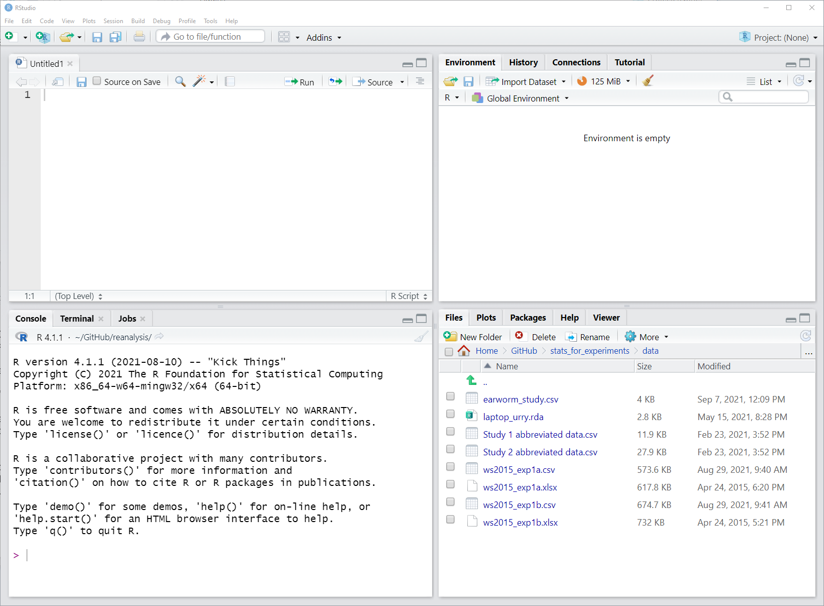
Figure 3.1: Screenshot of RStudio window with empty R script and default layout. The script is shown top left, the R console bottom left, the Environment pane in the top right, and the Files and Plot viewer in the bottom right.

This screenshot shows the four panes in their default location. The R script in the top left, the R console in the bottom left, the environment and history pane in the top right, and the files and plot pane in the bottom right.

An alternative to the default location is possible by switching the position of the console and environment pane. For this, click on the small button to the left of Addins just below the menu bar. The button looks a bit like a version of the windows logo. When clicking this button you can choose between the default "console on the left" and an alternative "console on the right". Especially if you work a lot with R scripts, which we will do, it makes sense to put the console on the right, as shown in the Figure 3.2.

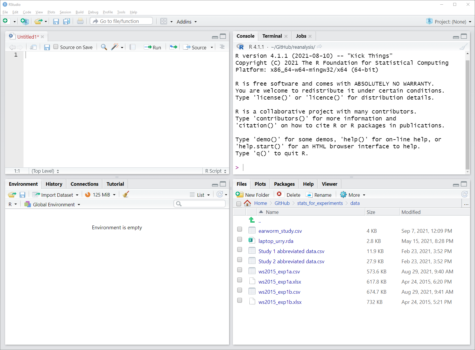
Figure 3.2: Screenshot of RStudio window with empty R script and alternative layout. In this image, console and environment pane have switched their position which allows both R script and console to occupy a larger space.

The benefit of using an R script is that you can come back to your code and change or rerun it. Even if you do not plan to save the R script, development is often easier in the script than directly in the console. Furthermore, one great thing about the R scripts and RStudio is that you can send commands from the R script directly to the R console using a keyboard shortcut: Ctrl + Enter on Windows/Linux and CMD + Enter on Mac. From here on in, we will indicate these options like this: Ctrl/CMD + Enter. Try it out yourself by typing something in the R script window (e.g., 7 + 3) and send it to the console using the shortcut. Let us now do some R.

3.4 A Base R Example Session

As we have discussed in the previous chapter, the most important format of data representation is a tabular format with each column representing a single variable and typically one row per observation. Such data is represented in base R in a data.frame, the most important data format for our needs. We use the term "base R" here to refer to using R without any additional packages. Let's quickly recap what a data.frame in base R looks like, and do some basic operations with it. This will also set the stage for using R scripts.

3.4.1 Data Files, Scripts, and Working Directory

In this chapter, we are mainly working with the data from Walasek and Stewart (2015), as introduced in detail in Section 1.2.2. The data consists of two data files, each representing a separate experiment, but which we have discussed together so far, as they are exact replications of one another. In Walasek and Stewart (2015) these are reported as Experiments 1a and 1b. The original data files sent to me by Lukasz Walasek were Excel files (which can be found here: Experiment 1a and Experiment 1b).

As base R does not allow to read in Excel files, I have opened the original data files of Walasek and Stewart (2015) in Excel and saved them as .csv files (comma separated value files) which can be downloaded from here: Experiment 1a and Experiment 1b. I recommend you download these files and save them in some folder so you can access them from within R. If you have problem downloading these files, try clicking on the links with the right mouse button (on Windows/Linux) or CMD + click (on Mac OS) and select "Save link as..." (or something similar to that) in the menu that appears. Note that if you click on .csv files on your computer, they will open in Excel (or an equivalent program), in case you wanted to have a look at them outside R.

In particular, I recommend the following steps so you can follow along with the upcoming R code:

• Save the downloaded data files in a folder named data that is in your current R working directory.
• Create a new empty R script and save it in the working directory.
• For example, say you already have created a folder for this book/class, let's assume this folder is called stats_r_intro-stuff and in some easy to find location (e.g., depending on your operating system the My Documents folder or your home folder ~). Let's assume you want this folder to be your working directory. Then, you create a new folder in this folder, called data (i.e., stats_r_intro-stuff/data), and download the two data files (Experiment 1a and Experiment 1b) into this folder. Next you create an empty R script in this folder for this chapter, say tidyverse-intro.R (i.e., it is now stats_r_intro-stuff/tidyverse-intro.R).
• You can now easily set your current R session to this folder as your working directory by opening tidyverse-intro.R in RStudio (if it is not yet opened) and the using the menu: Session - Set Working Directory - To Source File Location. This sets your working directory to the folder (i.e., location) in which the currently active R script is located, which should be your stats_r_intro-stuff folder. Note that if RStudio is not open, if you double-click on an R script file, RStusio will open and use the folder where your R script file is as the working directory (this only works if RStudio is not already running).
• Note, if you have been using the current R session already for some time, now is a good time to restart the session (not necessarily RStudio) by using the menu again: Session - Restart R.

The workflow laid out in the previous bullet points represents my general recommendation for working with R at this stage. Have a folder that is your designated project folder. In this folder you have your R scripts as well as a sub folder for the data. Then you can open a script in RStudio and set the folder to be your working directory through the menu (i.e., Session - Set Working Directory - To Source File Location). You can then access the data files simply by accessing data/my-data.file.csv. Importantly, don't forget to restart the R session before starting something new through the menu: Session - Restart R. You do not have to follow these steps if you find a different workflow that works better for you. The important thing is that you know what your working directory is and where your files are.

3.4.2 Read Data and Inspecting it

With this set-up steps out of the way, we can now load in the data from Experiment 1a using base R's read.csv() function:

df1a <- read.csv("data/ws2015_exp1a.csv")

This should read in the data file without any warnings or problems.²⁸ If for some reason you fail to download the file or fail to set the correct working directory, you can also try to read it directly from the internet as in the following code. But please only do that after you have tried downloading and dealing with the actual file. Handling data files and working with directories is an important R skill you need to acquire.

df1a <- read.csv("https://github.com/singmann/stats_for_experiments/raw/master/data/ws2015_exp1a.csv")

The first thing we usually want to do with a data.frame is to inspect its structure using the str() function, which lists all the variables, their data types, and the number of observations and variables.

str(df1a)
#> 'data.frame':    22912 obs. of  6 variables:
#>  $ subno    : int  8 8 8 8 8 8 8 8 8 8 ...
#>  $ loss     : int  6 6 6 6 6 6 6 6 8 8 ...
#>  $ gain     : int  6 8 10 12 14 16 18 20 6 8 ...
#>  $ response : chr  "accept" "accept" "accept" "accept" ...
#>  $ condition: num  20.2 20.2 20.2 20.2 20.2 20.2 20.2 20.2 20.2 20.2 ...
#>  $ resp     : int  1 1 1 1 1 1 1 1 0 1 ...

In the present case we have over 20 thousand observations on six variables. Most of the variables are int which means integer; that is, a numeric variable consisting solely of whole numbers (i.e., discrete values). We also have one num -- that is, numeric -- variable (i.e., numeric variable with decimal values), condition. In general, int and num variables are treated in the same way, as numeric variables, so there is hardly ever a reason to transform one into the other. Finally, condition is a chr or character variable.

3.4.3 Transforming Categorical Variables into Factors

As discussed in Section 2.2, some of the numeric variables as well as condition are actually categorical variables, or factors in R parlance. We can transform variables into factors using the aptly named factor() function. We generally use factor() instead of other functions (e.g., function as.factor()) because it allows us to specify the ordering of the factor levels and potentially other labels for the factor levels. Let us do so for three variables now, subno, response, and condition. For this we use the $ operator to access variables of a data.frame. After transforming the variables we take another look at the structure of the data.frame using str().

df1a$subno <- factor(df1a$subno)
df1a$response <- factor(df1a$response, levels = c("reject", "accept"))
df1a$condition <- factor(
  df1a$condition, 
  levels = c(40.2, 20.2, 40.4, 20.4), 
  labels = c("-$20/+$40", "-$20/+$20", "-$40/+$40", "-$40/+$20")
)
str(df1a)
#> 'data.frame':    22912 obs. of  6 variables:
#>  $ subno    : Factor w/ 358 levels "5","8","13","24",..: 2 2 2 2 2 2 2 2 2 2 ...
#>  $ loss     : int  6 6 6 6 6 6 6 6 8 8 ...
#>  $ gain     : int  6 8 10 12 14 16 18 20 6 8 ...
#>  $ response : Factor w/ 2 levels "reject","accept": 2 2 2 2 2 2 2 2 1 2 ...
#>  $ condition: Factor w/ 4 levels "-$20/+$40","-$20/+$20",..: 2 2 2 2 2 2 2 2 2 2 ...
#>  $ resp     : int  1 1 1 1 1 1 1 1 0 1 ...

We see that after running these commands, we have as expected three factors in the data. Let us take a look at each of these calls to factor() to understand why we call it in a different manner in each case.

• The call for subno only passes the variable (i.e., the df1a$subno vector) and no further arguments to factor(). As a consequence, the factor levels are ordered in an alpha-numerical increasing manner.

• The call for response specifies the ordering of the factor levels using the levels argument to which we have passed a vector of the levels, c("reject", "accept") (i.e., remember, c() is the function for creating vectors of any kind, such as character vectors here). The reason we do this is that otherwise the factor levels would be alphabetically ordered and then accept would be the first level and reject the second level (as "a" comes before "r" in the alphabet). This would be inconsistent with resp, where 0 = reject and 1 = accept.

• The call for condition specifies both the levels through levels as well as new names for the factor levels using labels. The labels use the ordering we have used throughout the book (i.e., potential loss first, potential gain second) and which differs from the ordering of the original condition (i.e., it switches the ordering to the format we are used to now). For both arguments a vector is passed, with elements mapped by position (i.e., the new label for the first level, 40.2, is the first label, -$20/+$40). We again specify the ordering of factor levels here through levels to maintain the ordering we have used throughout, with the condition that typically shows loss aversion, -$20/+$40 as first condition. If we had not done so, the first level would have been the -$20/+$20 condition (as 20.2 was the smallest number in the original vector).

An interesting part of the three calls to the factor() function is that if you run it again, after you have already run it, it will "break" the condition variable. If you try it out, you will see that all values of the condition variable change to NA if you run this call a second time. The reason for this is that the values passed through the levels argument need to be present in the variable. However, because we have replaced the original values with new labels, none of the original levels (i.e., c(40.2, 20.2, 40.4, 20.4)) is part of the variable any more. Consequently, all values are replaced by NA (i.e., "not available" which means missing data). To get the values back you need to reload the data using the read.csv() command from above and then you can run the factor() call again with the data in the same state it was when you ran it for the first time.

What this shows is that you cannot assume that running a piece of code twice gives the same output in all cases. The problem here is that the code changes the data itself (e.g., the values of condition). However, the code also assumes certain values for condition. Because this assumption only holds the first time you run the code, but not the second time, the second call breaks the results in somewhat unexpected ways. What this means is that randomly re-running code can lead to unexpected results (which are called "bugs" in programming language parlance). Therefore, instead of re-running individually pieces of code, it can often help to re-start at the top of a script and re-run everything in order to ensure all data is in the state you think it is (ideally after restarting the R session through Session - Restart R).

One more tip when transforming variables into factors. It is often a bit annoying to type out the factor levels by hand, especially when it is more than, say, two. In this case, a handy trick to know is that you can get R to produce the c() call having all factor levels. You just need to make sure you are using the correct ordering. The heart of the trick is the dput() function which creates a text representation of an R output that can be copied from the console to your script. To use this for factors the basic structure of the call is dput(unique(df$variable)) which returns the c() call for all unique elements of a variable. If you want the elements ordered you can use dput(sort(unique(df$variable))). For example, to create the levels argument for the condition variable I initially executed dput(sort(unique(df1a$condition))) at the console which returns c(20.2, 20.4, 40.2, 40.4) for the original df1a data (i.e., before turning everything into factors). I then just copied and pasted a bit in this vector to get the ordering right (admittedly, typing might have been faster than copying and pasting, but whatever).

Another thing we often want to do when reading in the data is getting an overview of what it actually looks like. One way to do this that I do not recommend for data.frames is just typing the name of the variable into the console (or calling just the name from the script). When you do this, the object is printed in the console window, which, for large data.frames, leads to hundreds or thousands of rows being printed until some printing limit is reached. An alternative is to just look at the first few rows using the head() function (which prints the first 6 rows per default):

head(df1a)
#>   subno loss gain response condition resp
#> 1     8    6    6   accept -$20/+$20    1
#> 2     8    6    8   accept -$20/+$20    1
#> 3     8    6   10   accept -$20/+$20    1
#> 4     8    6   12   accept -$20/+$20    1
#> 5     8    6   14   accept -$20/+$20    1
#> 6     8    6   16   accept -$20/+$20    1

Alternatively, you can click on an object in the RStudio "Environment" pane (see Figures 3.1 and 3.2) which opens the data in a viewer pane. The equivalent R call is using View(df1a) which opens the same viewer. However, View() should only be used interactively at the console and not be in an R script as it requires user interaction beyond script and console. In other words, View() is useful during development to get an overview of the data, but not for the final analysis script.

3.5 The tidyverse

A popular extension to base R is the tidyverse (Wickham et al. 2019), a selection of packages curated and in large parts developed by the RStudio company. The mastermind behind the tidyverse is Hadley Wickham, the RStudio chief scientist and maybe the one person that can be considered an R superstar.²⁹ Most of the core tidyverse packages that will be introduced below, such as dplyr and ggplot2, are his developments (even though many others have contributed to those packages as well).

As a reminder, packages are a collection of functions and other R objects (e.g., data) that provide additional functionality on top of base R. To be able to use a package, it needs to be installed from CRAN once before it can be loaded in your R session. The easiest way to install a package is using install.packages(). Note that it is a good idea to only run install.packages() at the console and not to put it into your R script. The reason for this is that you only want to execute install.packages() once per R installation or after updating R and not every time you run a script.

Therefore, we begin by installing the tidyverse package from CRAN using install.packages(). This will automatically install all the individual packages discussed below. As a reminder, this only needs to be done once and not everytime you run a script.

install.packages("tidyverse")

Then, you can load all tidyverse packages at once using the library() function. Loading the tidyverse package this way is something we will do at the top of pretty much all scripts we will be creating.

library("tidyverse")
#> ── Attaching core tidyverse packages ──── tidyverse 2.0.0 ──
#> ✔ dplyr     1.1.3     ✔ readr     2.1.4
#> ✔ forcats   1.0.0     ✔ stringr   1.5.0
#> ✔ ggplot2   3.4.3     ✔ tibble    3.2.1
#> ✔ lubridate 1.9.3     ✔ tidyr     1.3.0
#> ✔ purrr     1.0.2     
#> ── Conflicts ────────────────────── tidyverse_conflicts() ──
#> ✖ dplyr::filter() masks stats::filter()
#> ✖ dplyr::lag()    masks stats::lag()
#> ℹ Use the conflicted package (<http://conflicted.r-lib.org/>) to force all conflicts to become errors

When loading packages it is common that this produces some status or other messages in the console (some packages do, some don't). For example, tidyverse lists the package versions of the loaded (or "attached") packages and lists function conflicts; that is, cases in which a tidyverse function masks a previous loaded function with the same name. We include these messages here to show that this is normal and nothing to worry about, but will generally not later in the book, as this would get repetitive. However, note that the exact version numbers of the packages that are shown here may differ from the version numbers you see, simply because some packages might be updated after this book was written.

The core tidyverse packages are (with descriptions taken or adapted from the official websites):

• tibble: A modern version of the data.frame

• readr: For reading in data the RStudio way.

• Data wrangling with magrittr, tidyr, and dplyr: A coherent set of functions for tidying, transforming, and working with rectangular (i.e., tabular) data. Supersedes many base R functions and makes common data manipulations very easy.

• ggplot2: A system for data visualization, in other words, making graphs. This will be discussed in the next chapter.

• purr and broom: Advanced modelling with the tidyverse and tidymodels which will not be discussed here.

In the following we provide a short introduction to the core components of the tidyverse as they are needed for this book. A more comprehensive introduction is provided in the Wickham and Grolemund book "R for Data Science" which is available freely at http://r4ds.had.co.nz. To get a good grip on the tidyverse, I highly recommend working through chapters 1 to 21, or better still, to chapter 25 (the chapters in "R for Data Science" are a lot shorter than the chapters in the present book).

3.5.1 tibble and readr

The back bone of the tidyverse is the tibble, or tbl_df (it's class name in R), "a modern reimagining of the data.frame, keeping what time has proven to be effective, and throwing out what is not" (quote from tibble documentation). The main difference between a data.frame and tibble in daily use is that tibbles do not try to print all rows and columns and thus do not overwhelm the console when just entering the name of the data at the console. This feature alone is enough for me to prefer tibbles over data.frames. When working on an analysis, one often wants to have a quick look at the data to see what has happened and the easiest way to do that is often to just enter the name of the data into the console.

To convert a data.frame into a tibble you can use the as_tibble() function. Let's do this for our existing data.frame of Walasek and Stewart (2015), df1a.

tbl1a <- as_tibble(df1a)
tbl1a
#> # A tibble: 22,912 × 6
#>   subno  loss  gain response condition  resp
#>   <fct> <int> <int> <fct>    <fct>     <int>
#> 1 8         6     6 accept   -$20/+$20     1
#> 2 8         6     8 accept   -$20/+$20     1
#> 3 8         6    10 accept   -$20/+$20     1
#> 4 8         6    12 accept   -$20/+$20     1
#> 5 8         6    14 accept   -$20/+$20     1
#> 6 8         6    16 accept   -$20/+$20     1
#> # ℹ 22,906 more rows

In the output of the tibble, we can see two things. First, the output only shows the first 6 rows. Compare this to what happens when typing df1a in the console which will print many more rows (so you cannot see the column names anymore). Second, the data type of each column is shown below the column names. This is another feature that makes tibbles more convenient in everyday use. We directly see that for example subno is a factor (<fct>) as it should be.

An alternative way to create a tibble instead of a standard data.frame is by loading the data using the tidyverse specific read functions which are in the readr package. Remember that above we used the base R read function read.csv(), which is one of a handful of base R data read functions such as read.table() (for reading data separated by spaces) and read.delim() (for reading tab separated data). readr offers a similar set of functions where the main differences are that instead of using a . in the function name they use an _ and instead of a data.frame they return a tibble. So in case you have a csv file, you could use read_csv() instead of read.csv(). Note that in this and in the following code chunks, we are going to overwrite the existing tbl1a object to not clutter the work space.

tbl1a <- read_csv("data/ws2015_exp1a.csv")
#> Rows: 22912 Columns: 6
#> ── Column specification ────────────────────────────────────
#> Delimiter: ","
#> chr (1): response
#> dbl (5): subno, loss, gain, condition, resp
#> 
#> ℹ Use `spec()` to retrieve the full column specification for this data.
#> ℹ Specify the column types or set `show_col_types = FALSE` to quiet this message.
tbl1a
#> # A tibble: 22,912 × 6
#>   subno  loss  gain response condition  resp
#>   <dbl> <dbl> <dbl> <chr>        <dbl> <dbl>
#> 1     8     6     6 accept        20.2     1
#> 2     8     6     8 accept        20.2     1
#> 3     8     6    10 accept        20.2     1
#> 4     8     6    12 accept        20.2     1
#> 5     8     6    14 accept        20.2     1
#> 6     8     6    16 accept        20.2     1
#> # ℹ 22,906 more rows

What we can see from the output is that read_csv() not only returns the tibble, but also a message showing the column specification (i.e., data type for each column). We could use this to change the column type when reading in the data, but I usually do not find this necessary. In most cases it is sufficient to change the data type once the data is read in, as shown below.

As the status message also shows, you can stop this message from appearing by specifying an additional argument to the read_csv() call, show_col_types = FALSE. I don't think this is necessary. However, the following shows that it works as expected.

tbl1a <- read_csv("data/ws2015_exp1a.csv", show_col_types = FALSE)
tbl1a
#> # A tibble: 22,912 × 6
#>   subno  loss  gain response condition  resp
#>   <dbl> <dbl> <dbl> <chr>        <dbl> <dbl>
#> 1     8     6     6 accept        20.2     1
#> 2     8     6     8 accept        20.2     1
#> 3     8     6    10 accept        20.2     1
#> 4     8     6    12 accept        20.2     1
#> 5     8     6    14 accept        20.2     1
#> 6     8     6    16 accept        20.2     1
#> # ℹ 22,906 more rows

Another feature of readr compared to the corresponding base R functions is that it is a bit more restrictive in some cases. That is, in case the data is not as expected by a particular read function, readr fails more often than base R. Whereas this can appear annoying while programming, it has the benefit that one learns of problems in the data early compared to late. In other words, readr functions are more likely than base R functions to ensure the data looks like you expect it to. And if your data is more likely to look like you expect it to, your code will be less likely to produce incorrect results.

Therefore, in addition to using read_csv() instead of read.csv(), it is often better to use read_table() instead of read.table() for space separated data (or read_table2() if the data format is a bit sloppy), read_tsv() instead of read.delim() for tab separated data, or read_delim() if you want to specify the data delimiter.

3.5.2 The Pipe: %>%

One of the coolest, and at the time novel (for R), features of the tidyverse is the pipe, which is the name of the %>% operator.³⁰ To understand what it does and why it is so great, it makes sense to begin by taking a step back and thinking a bit about functions and evaluation order in R.

One of the most important features of R is that we can take the result (or output) from one operation and use it as the input of another operation. For example, remember that the loss column in the data of Walasek and Stewart (2015) shows the potential loss for each of the lotteries, ranging from $6 to $40. Now imagine that we want to know the midpoint between the minimum and maximum loss (which is $23 in the present case). One way to calculate those is by taking the mean of the minimum and maximum. To get this in R we would need to do two steps: get the minimum and maximum potential loss from the vector of losses and then take the mean of the minimum and maximum. We can get the minimum and maximum of a vector using the range() function and the mean is obtained using the mean() function. So to do so in R for our vector of all potential losses, tbl1a$loss, we could do:

# step 1: get minimum and maximum and save in temporary variables
tmp <- range(tbl1a$loss)
tmp # print minimum and maximum, to check everything is okay
#> [1]  6 40
#step 2: calculate mean of minimum and maximum:
mean(tmp)
#> [1] 23

This code above does this two-step calculation explicitly and saves the results of the first step in a temporary variable we have called tmp. We could also combine both steps into one by passing the results of the first step to the mean() function:

mean(range(tbl1a$loss))
#> [1] 23

We first get the minimum and maximum (i.e., the range) and then pass this to the mean() function. As the mean function is the last operation we want, it is the outermost call in this line of code. In other words, in R code that does not use the pipe, code is executed from the inside to the outside. This can make it difficult to chain many operations after each other without the need to create temporary variables as we did first.

In contrast to executing code from innermost to outermost, the pipe allows us to chain operations from left to right. We can start with the innermost call and pipe it to the next function using %>%. For example, using the pipe we could do the following:

tbl1a$loss %>% 
  range() %>% 
  mean()
#> [1] 23

This shows a typical pipe workflow. We start with our data, in the present case the tbl1a$loss vector. This data is piped to the first operation, the range() function. The output of this call is piped to the next operation, the mean() function. At the end, we get exactly the output we should get but with code that is easier to read. One feature of the pipe that makes the code particularly readable is that we can start a new line for each step in a chain.

The pipe also works like any regular R operation, so we can easily save the result from the whole chain of operation in a new object for later use. For example:

loss_midpoint <- tbl1a$loss %>%
  range() %>% 
  mean()
loss_midpoint
#> [1] 23

To sum this up again, in base R the order of operations is from the innermost to the outermost. With the pipe, in contrast, we can chain (or pipe) operations from left to right. The following image exemplifies this using a screenshot of a slide from Andrew Heiss. In the top part we see the operations me needs to execute in order to leave the house using base R (i.e., starting with the innermost wakeup() function). The coding style without the pipe makes it difficult to see what happens when, and is generally difficult to read, not least because it is hard to see which function arguments (like pants=TRUE) go with which function (like get_dressed). The lower part shows the same operations using the pipe. We can see how much easier it is to see the logic from waking up, getting out of bed, and so forth, not to mention which arguments go with which function.

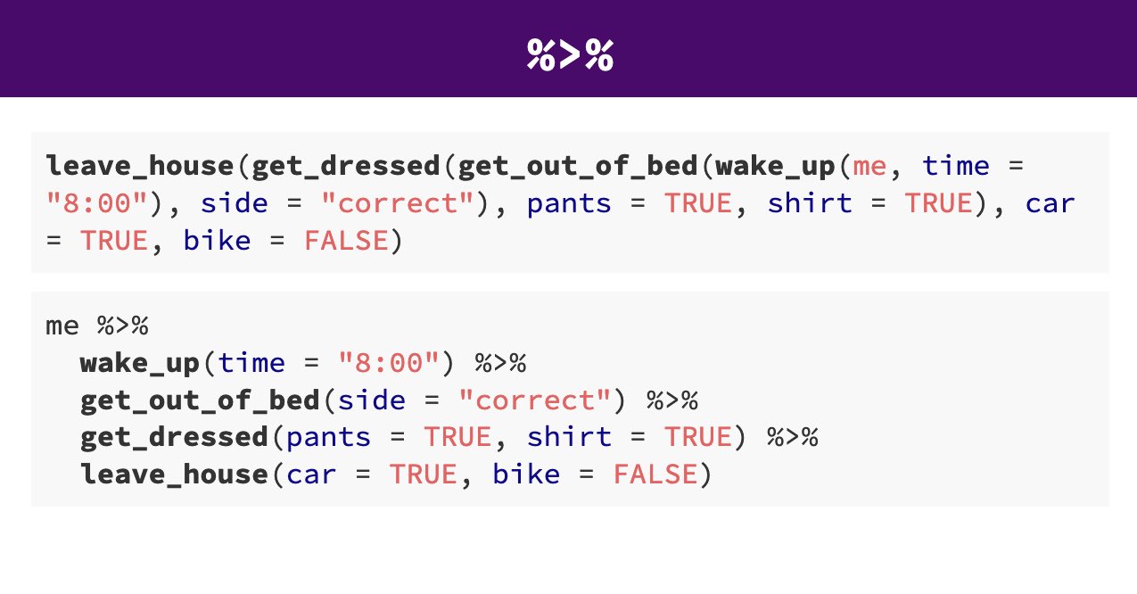
Figure 3.3: Comparison of execution order without pipe (upper part) or with pipe (lower part). From: https://evalsp21.classes.andrewheiss.com/projects/01_lab/slides/01_lab.html#116

In the following sections we will see how powerful piping can be. We can do quite a lot of neat things relatively easily, especially when the pipe is combined with the dplyr functions that will be introduced next.

Let us end this section with two more points that are important. First, typing the pipe (i.e., typing the characters %>%) is annoying. If you are in RStudio, there is an alternative, in the form of a keyboard shortcut: Ctrl/Cmd + Shift + M. I highly recommend you get used to using this shortcut. It is one of the few shortcuts in RStudio I use regularly.³¹

Second, base R now has its own pipe, |>. It works very similarly to the tidyverse pipe (and can in many situations be used instead of the tidyverse pipe) and can be used without loading any packages. I am not using it here for the only reason that I have adapted the tidyverse pipe before there was a base R pipe and there does not seem to be many reasons to prefer one over the other if the tiydverse is already loaded. So if you see |> instead of %>% somewhere, assume it does pretty much the exact same thing.

3.5.3 dplyr

Whereas the back bone of the tidyverse are the tibble and the pipe, the package that most significantly improves one's workflow is dplyr (pronounced dee-plier, like the tool). There are five core functions of dplyr which, together, provide the most common data manipulation operations. Or to quote the official documentation: "dplyr is a grammar of data manipulation, providing a consistent set of verbs that help you solve the most common data manipulation challenges." These five verbs/functions are:

• mutate() adds new variables or changes variables as a function of existing variables
• select() picks variables based on their names
• filter() picks cases based on their values
• summarise() reduces multiple values down to a summary
• arrange() changes the ordering of the rows

A great introduction and overview of the functionality of these functions is provided on the official getting started page, but we will do so here as well, if only somewhat briefly.

One important point is that all dplyr functions work with what is called non-standard evaluation. This means we can refer to variable names of the data.frame/tibble we are working with in any of the dplyr functions without enclosing them in quotes. If this sounds a bit mysterious to you, remember that the only thing we can usually refer to without quotes are R objects that exist in the workspace (i.e., objects listed in the environment pane in RStudio). As variables in tibbles/data.frames are no objects itself, but only exist in the context of the data.frame/tibble, many of the functions we will get to know in later packages require their names to be enclosed in quotes. However, this is generally not the case for tidyverse functions saving a few keystrokes.

Finally, all dplyr functions work with the pipe, so can be chained.

3.5.3.1 mutate()

As an example, here is how you can use mutate() and the pipe to convert some variables in a data set to factors, as we did above in base R. We start again by reading the data in. We then pipe this data to the mutate() function to convert three variables to factors as done above, and save it again in the same object, tbl1a. We then get an overview of the object.

tbl1a <- read_csv("data/ws2015_exp1a.csv")
tbl1a <- tbl1a %>% 
  mutate(
    subno = factor(subno),
    response = factor(response, levels = c("reject", "accept")),
    condition = factor(
      condition, 
      levels = c(40.2, 20.2, 40.4, 20.4), 
      labels = c("-$20/+$40", "-$20/+$20", "-$40/+$40", "-$40/+$20")
    )
  )
tbl1a
#> # A tibble: 22,912 × 6
#>   subno  loss  gain response condition  resp
#>   <fct> <dbl> <dbl> <fct>    <fct>     <dbl>
#> 1 8         6     6 accept   -$20/+$20     1
#> 2 8         6     8 accept   -$20/+$20     1
#> 3 8         6    10 accept   -$20/+$20     1
#> 4 8         6    12 accept   -$20/+$20     1
#> 5 8         6    14 accept   -$20/+$20     1
#> 6 8         6    16 accept   -$20/+$20     1
#> # ℹ 22,906 more rows

You can see a number of changes here as compared to the base R code:

• The block of code in which variables are converted to factors is wrapped into the mutate() call to which we have piped the data, tbl1a.
• For each operation that converts one variable to a factor, we use the = sign and not the assignment operator <-, because all the operations are performed within the mutate() function. We generally only use the assignment operator <- outside of function calls (if you try it out and replace the = with <- you will see what horrible consequences this has).
• The first two calls for changing a variable finish with a ,, again because we are inside one mutate() call. The , tells mutate() we are not yet done specifying a set of operations.
• Instead of passing the full vector to factor() (as we did above using df1a$subno), we can refer to each variable, such as subno, by name (and without quotes) directly (this is what is meant by non-standard evaluation). Again, this arises from the fact that we are working within the context of the data set that we originally piped to the mutate() call.

3.5.3.2 summarise()

The second most important function from dplyr is summarise() which as the name suggests, creates summaries. This means that we are reducing the number of rows in a data set to one row (or one row per grouping variable, as explained below). For example, we could use summarise() to get the average probability with which lotteries were accepted across all conditions and lotteries. For this, we just need to take the overall mean of the resp variable.

tbl1a %>% 
  summarise(mean_acc = mean(resp))
#> # A tibble: 1 × 1
#>   mean_acc
#>      <dbl>
#> 1    0.381

We see that summarise() also returns a tibble, so the values returned differ quite a bit from what one would get in base R (using mean(tbl1a$resp)). We can also see that summarise() works structurally quite similarly to mutate(). In the summarise() call, we can create new variables using a name = operation syntax. We can also create multiple summary statistics by separating them using ,. We can also add comments to the code as usual using #, as long as it is to the right side of the ,.

tbl1a %>% 
  summarise(
    mean_acc = mean(resp),
    sd_acc = sd(resp),  ## sd() returns the standard deviation
    mean_pot_loss = mean(loss),
    mean_pot_gain = mean(gain)
  )
#> # A tibble: 1 × 4
#>   mean_acc sd_acc mean_pot_loss mean_pot_gain
#>      <dbl>  <dbl>         <dbl>         <dbl>
#> 1    0.381  0.486          19.5          19.2

3.5.3.3 filter(), select(), and arrange()

As we have discussed above, one of the key ways of using the tidyverse is by chaining different operations together. For example, we could first create a data set of observations from the "-$20/+$40" condition only, and then calculate summaries for this condition alone. For this, we pipe first to the filter() function, and then pipe the results to summarise():

tbl1a %>%
  filter(condition == "-$20/+$40") %>% 
  summarise(
    mean_acc = mean(resp),
    sd_acc = sd(resp),
    mean_pot_loss = mean(loss),
    mean_pot_gain = mean(gain)
  )
#> # A tibble: 1 × 4
#>   mean_acc sd_acc mean_pot_loss mean_pot_gain
#>      <dbl>  <dbl>         <dbl>         <dbl>
#> 1    0.514  0.500            13            26

Note that filter() requires the use of the == operator and not the = operator. The reason is that you do not want to set a variable equal to something, which is done using =, but want to check for equality, which is done using ==. filter() also allows you to chain multiple comparisons together, either by separating them using , or & (i.e., logical and). If only one of multiple conditions needs to hold, you can use | (logical or).

filter() is also the function for removing observations. This is done by writing a filter that retains all observations except for the ones you want to remove. For this you can also use the logical not operator, ! which inverts a logical vector, or the unequal operator, !=.

For example, you'll recall that, with relation to the study of Walasek and Stewart (2015), what we are actually interested in are the responses to the symmetric lotteries (when the potential loss is equal to the potential gain). We could select those with filter():

symm1 <- tbl1a %>%
  filter(loss == gain)
symm1
#> # A tibble: 1,989 × 6
#>   subno  loss  gain response condition  resp
#>   <fct> <dbl> <dbl> <fct>    <fct>     <dbl>
#> 1 8         6     6 accept   -$20/+$20     1
#> 2 8         8     8 accept   -$20/+$20     1
#> 3 8        10    10 accept   -$20/+$20     1
#> 4 8        12    12 accept   -$20/+$20     1
#> 5 8        14    14 accept   -$20/+$20     1
#> 6 8        16    16 accept   -$20/+$20     1
#> # ℹ 1,983 more rows

Or equivalently:

symm2 <- tbl1a %>%
  filter(!(loss != gain))
all.equal(symm1, symm2)
#> [1] TRUE

Here, we use the all.equal() function to show that the two objects are the same. This function can compare arbitrary R objects and only returns TRUE if two objects are identical.

One problem with the filter() command used above is that it selects all symmetric lotteries and not only the symmetric lotteries that appear in all conditions. In other words, it also selects some symmetric lotteries that only appear in a subset of the conditions. As our goal is to compare performance across conditions -- for this to be a fair comparison it needs to be done on only the lotteries that are shared across all conditions -- this filter() call is therefore not the correct one. The following code, which shows all symmetric lotteries for each condition, demonstrates this.

tbl1a %>%
  filter(loss == gain) %>% 
  select(loss, gain, condition) %>% 
  unique() %>% 
  arrange(condition) %>% 
  print(n = Inf)
#> # A tibble: 22 × 3
#>     loss  gain condition
#>    <dbl> <dbl> <fct>    
#>  1    12    12 -$20/+$40
#>  2    16    16 -$20/+$40
#>  3    20    20 -$20/+$40
#>  4     6     6 -$20/+$20
#>  5     8     8 -$20/+$20
#>  6    10    10 -$20/+$20
#>  7    12    12 -$20/+$20
#>  8    14    14 -$20/+$20
#>  9    16    16 -$20/+$20
#> 10    18    18 -$20/+$20
#> 11    20    20 -$20/+$20
#> 12    12    12 -$40/+$40
#> 13    16    16 -$40/+$40
#> 14    20    20 -$40/+$40
#> 15    24    24 -$40/+$40
#> 16    28    28 -$40/+$40
#> 17    32    32 -$40/+$40
#> 18    36    36 -$40/+$40
#> 19    40    40 -$40/+$40
#> 20    12    12 -$40/+$20
#> 21    16    16 -$40/+$20
#> 22    20    20 -$40/+$20

In particular, the output shows that in the asymmetric conditions, -$20/+$40 and -$40/+$20, we only have three symmetric lotteries, whereas in the two symmetric conditions we have quite a lot more. However, the three symmetric lotteries that appear in the asymmetric conditions, 12-12, 16-16, and 20-20, appear in all conditions.

Before focussing on how we can build a better filter, let's first examine in detail how the code above works. We first filter to obtain all symmetric lotteries. From this data set, we then retain or select() only the loss, gain, and condition columns. We then use the unique() function to only retain the unique rows. Because we have a specific ordering in which we think about the conditions (which is expressed in the order of the factor levels) we then sort the tibble along the condition variable using arrange(). Finally, because a tibble only prints a few rows by default, we use print(n = Inf) which prints all rows (i.e., up to row infinity).

To better understand the code, you are encouraged to run it line by line to see what the output at each intermediate step is. The easiest way to do so is by selecting parts of it in the R script window and then sending it to the console using the shortcut (i.e., Ctrl/CMD + Enter). Note that when selecting only a subset of lines in this code, do not select the %>% at the end of the last line before sending it to the console. Otherwise R will think you are not yet finished. In general, it's a good idea to step line-by-line through much of the code we present here, and at your own speed, in order to fully understand its operation.

Now that we know which symmetric lotteries there are, how can we select only the symmetric lotteries that appear in all conditions? There clearly are multiple different filters that would do this. The one that first comes to my mind is to combine the filter that selects all symmetric lotteries with a filter that only selects lotteries in which the potential loss is either 12, 16, or 20. For the latter, we introduce a new operator, the %in% operator. It returns TRUE for any element of a vector that matches an element in another vector. For example in our case, we want to retain all those lotteries where the potential loss is in c(12, 16, 20). This is shown below. We also include the code that shows we now have the same set of symmetric lotteries in all conditions.

tbl1a %>%
  filter(loss == gain, loss %in% c(12, 16, 20)) %>% 
  select(loss, gain, condition) %>% 
  unique() %>% 
  arrange(condition) 
#> # A tibble: 12 × 3
#>    loss  gain condition
#>   <dbl> <dbl> <fct>    
#> 1    12    12 -$20/+$40
#> 2    16    16 -$20/+$40
#> 3    20    20 -$20/+$40
#> 4    12    12 -$20/+$20
#> 5    16    16 -$20/+$20
#> 6    20    20 -$20/+$20
#> # ℹ 6 more rows

3.5.3.4 group_by()

You might remember that the main hypothesis of Walasek and Stewart (2015) was that it is not the absolute value of a lottery, but its relative rank, that matters for whether or not participants think a lottery is attractive. The main evidence for this hypothesis was that the proportion with which the symmetric lotteries are accepted differs across the four conditions. How canwe calculate this with the tiydverse?

Only applying what we know so far, we would split the data into four subsets using filter(), and then apply summarise() to each of these subsets. Let's show how this would work by only splitting the data into two subsets, one for the "-$20/+$40" condition that shows loss aversion and one for the "-$40/+$20" condition that shows loss seeking. We need to combine this filter with the filter selecting only the symmetric lotteries. To make the logic easier, we separate these two steps into separate filter() calls (but could also combine them into one).

## "loss aversion" condition:
tbl1a %>%
  filter(loss == gain, loss %in% c(12, 16, 20)) %>% 
  filter(condition == "-$20/+$40") %>% 
  summarise(mean_acc = mean(resp))
#> # A tibble: 1 × 1
#>   mean_acc
#>      <dbl>
#> 1    0.167

## "loss seeking" condition:
tbl1a %>%
  filter(loss == gain, loss %in% c(12, 16, 20)) %>% 
  filter(condition == "-$40/+$20") %>% 
  summarise(mean_acc = mean(resp))
#> # A tibble: 1 × 1
#>   mean_acc
#>      <dbl>
#> 1    0.670

The results show the previously discussed pattern. Participants in the -$20/+$40 condition are around 50 percentage points less likely to accept the symmetric lotteries than participants in the -$40/+$20 condition. Whereas this analysis clearly does what we want it to do, the code is a bit verbose and clunky. For example, the first filter() call and the summarise() call are identical in both parts. So the question is: Is there not a better way to get these results?

This is, of course, a rhetorical question and the answer is yes, there is a better way. The answer is the group_by() function, the function that gives dplyr its full power. To use group_by(), you need to pass it one or multiple (categorical) grouping variables. group_by() then creates a grouped tibble with the consequence that if any of the further dplyr verbs are applied to this grouped tibble, they are applied to each group separately. Let's show it for our example to see what this means in practice:

tbl1a %>%
  filter(loss == gain, loss %in% c(12, 16, 20)) %>% 
  group_by(condition) %>% 
  summarise(mean_acc = mean(resp))
#> # A tibble: 4 × 2
#>   condition mean_acc
#>   <fct>        <dbl>
#> 1 -$20/+$40    0.167
#> 2 -$20/+$20    0.462
#> 3 -$40/+$40    0.437
#> 4 -$40/+$20    0.670

We can see that the output now contains the average proportion of accepting the symmetric lotteries for each of the four conditions separately. So instead of first splitting the data and then calculating the summary statistics (here, the mean of the resp column) for each split separately, group_by() does exactly this internally.

In other words, whenever we have a categorical variable in our data, we can use group_by() to perform operations separately across the levels of the categorical variable. Given the ubiquity of categorical variables -- for example, every experiment has at least one experimental factor -- this is a huge time and effort saver.

And whereas here we have shown the use of group_by() for summarise() (which is probably the most common use), group_by() also works for the other dplyr verbs for which the results can depend on other rows, mutate() and arrange().

In the example above, we have only passed one variable (condition) to group_by(). But we can also pass multiple variables. This will perform the operations conditional on the combination of both variables. For example, here we have selected the three symmetric lotteries that are the same across conditions. With group_by(), it is easy to get the average proportion of acceptances separately for each lottery and condition. As this returns a tiible with more rows as shown by default, we again use print(n = Inf) as the last command in the pipe chain to show all rows.

tbl1a %>%
  filter(loss == gain, loss %in% c(12, 16, 20)) %>% 
  group_by(condition, loss, gain) %>% 
  summarise(mean_acc = mean(resp)) %>% 
  print(n = Inf)
#> `summarise()` has grouped output by 'condition', 'loss'.
#> You can override using the `.groups` argument.
#> # A tibble: 12 × 4
#> # Groups:   condition, loss [12]
#>    condition  loss  gain mean_acc
#>    <fct>     <dbl> <dbl>    <dbl>
#>  1 -$20/+$40    12    12    0.190
#>  2 -$20/+$40    16    16    0.119
#>  3 -$20/+$40    20    20    0.190
#>  4 -$20/+$20    12    12    0.469
#>  5 -$20/+$20    16    16    0.458
#>  6 -$20/+$20    20    20    0.458
#>  7 -$40/+$40    12    12    0.448
#>  8 -$40/+$40    16    16    0.437
#>  9 -$40/+$40    20    20    0.425
#> 10 -$40/+$20    12    12    0.681
#> 11 -$40/+$20    16    16    0.659
#> 12 -$40/+$20    20    20    0.670

Note that pretty much the same result would be obtained if only passing one of the gain/loss variable pairs to group_by() here (i.e., group_by(condition, loss) or group_by(condition, gain)). Feel free to try it out.

These results are not straightforward to interpret as they do not show a consistent pattern across conditions. For the symmetric conditions, the difference in acceptance rate seems to be small. However, for the asymmetric conditions, we see somewhat larger differences, suggesting that the 16-16 lottery may have somewhat lower acceptance rates than both the 12-12 and 20-20 lottery. As these are only descriptive results without any additional statistical evidence, it is very much possible that these small differences within conditions reflect pure noise and should not be taken too seriously.

Before moving to the next function, there is one more thing to discuss. As shown in the output above, summarise() returns a tibble that is still grouped due to the call to the group_by() command with more than one variable. This can be seen by both the status message "summarise() has grouped output by ..." and because the output still shows # Groups: .... This means that if we were to do any further operations on this tibble, it would still be performed grouped. To remove the grouping created by group_by(), use ungroup():

tbl1a %>%
  filter(loss == gain, loss %in% c(12, 16, 20)) %>% 
  group_by(condition, loss, gain) %>% 
  summarise(mean_acc = mean(resp)) %>% 
  ungroup()
#> `summarise()` has grouped output by 'condition', 'loss'.
#> You can override using the `.groups` argument.
#> # A tibble: 12 × 4
#>   condition  loss  gain mean_acc
#>   <fct>     <dbl> <dbl>    <dbl>
#> 1 -$20/+$40    12    12    0.190
#> 2 -$20/+$40    16    16    0.119
#> 3 -$20/+$40    20    20    0.190
#> 4 -$20/+$20    12    12    0.469
#> 5 -$20/+$20    16    16    0.458
#> 6 -$20/+$20    20    20    0.458
#> # ℹ 6 more rows

3.5.3.5 Counting

Another important functionality of dplyr is that it makes it easy to count observations using the count() or n() functions. Counting is one of the operations that seems somewhat unspectacular at the beginning, but is extremely important for understanding your data. For example, an important question we might have for our data is how many participants we have per condition or how many trials every participant worked on. Counting is also a good way to check that you have the exact number of observations that you expect from the original design of the experiment.

Let us begin by looking at the number of trials per participant (and condition). There are two almost equivalent ways of doing this, either using group_by() and summarise(n = n()) or count():

tbl1a %>% 
  group_by(condition, subno) %>% 
  summarise(n = n())
#> `summarise()` has grouped output by 'condition'. You can
#> override using the `.groups` argument.
#> # A tibble: 358 × 3
#> # Groups:   condition [4]
#>   condition subno     n
#>   <fct>     <fct> <int>
#> 1 -$20/+$40 5        64
#> 2 -$20/+$40 13       64
#> 3 -$20/+$40 53       64
#> 4 -$20/+$40 61       64
#> 5 -$20/+$40 73       64
#> 6 -$20/+$40 85       64
#> # ℹ 352 more rows

tbl1a %>% 
  count(condition, subno)
#> # A tibble: 358 × 3
#>   condition subno     n
#>   <fct>     <fct> <int>
#> 1 -$20/+$40 5        64
#> 2 -$20/+$40 13       64
#> 3 -$20/+$40 53       64
#> 4 -$20/+$40 61       64
#> 5 -$20/+$40 73       64
#> 6 -$20/+$40 85       64
#> # ℹ 352 more rows

We can see that the results are pretty much the same, the only difference being that group_by() retains the grouped tibble whereas count() does not.

We can also see that the number of trials for each of the participants shown in the output is 64. This is exactly the number of trials we would expect from the description of the study in Section 1.2.2. However, so far we cannot be sure that this really holds for all participants. We expect this to be the case and it looks like it for a handful of participants shown, but does it really hold for everyone?

When analysing data, questions such as these regularly come to one's mind. One has assumptions about what the data should look like, but one cannot be sure that these assumptions really hold. What if, for example, data collection did not finish for some participants and we only have partial data for those? The reality of analysing actual data is that often some assumptions one has about the data set do not hold. Many things can and will go wrong during data collection, so an important step in any analysis is to verify one's assumptions.

So how can we check if everyone has exactly 64 trials? With the code above, this can be done per group by extending it with another group_by() summarise() combination. This also allows us to count, in the same step, the number of participants in each condition:

tbl1a %>% 
  group_by(condition, subno) %>% 
  summarise(n = n()) %>% 
  group_by(condition) %>% 
  summarise(
    n_participants = n(),
    all_64 = all(n == 64)
  )
#> `summarise()` has grouped output by 'condition'. You can
#> override using the `.groups` argument.
#> # A tibble: 4 × 3
#>   condition n_participants all_64
#>   <fct>              <int> <lgl> 
#> 1 -$20/+$40             84 TRUE  
#> 2 -$20/+$20             96 TRUE  
#> 3 -$40/+$40             87 TRUE  
#> 4 -$40/+$20             91 TRUE

So what exactly is happening here? After the first three lines (including the first summarise()), we create the once summarised tibble already shown in the previous code. This tibble has one row per participant with the n column giving the number of trials for that participant. We then group this tibble again by condition to ensure the following results are shown separately for each condition (which is not really necessary, as it is still grouped by condition, but makes the code clearer). We then perform another summarise() which summarises the once summarised tibble for each condition. In this summarise(), we perform two operations:

1. We create a new variable n_participants, which contains the number of observations (number of participants) in the once summarised tibble. This is done as before using the n() function for counting observations.
2. We create a new logical variable all_64, which is TRUE only if for all observations/participants within one condition the number of trials is 64. To fully understand the call creating this variable, we have to read it from the inside to the outside. The innermost call is n == 64. This creates a logical variable for each observation in the once summarised tibble that is TRUE if the number of trials (the variable n) is 64 and FALSE otherwise. Then we pass this vector to the all() function which reduces a logical vector to a single logical variable. all() only returns TRUE if all elements of the vector are TRUE and FALSE otherwise.

The results thus show two pieces of information per condition. First, we can see the number of participants per condition, which is between 84 and 96. Second, for all conditions, all participants have exactly 64 trials, as indicated by the values of the all_64 vector being TRUE for all conditions.

3.5.3.6 dplyr Summary

We have seen that dplyr is a powerful tool for working with data.frames or tibbles. The five verbs, mutate(), summarise(), filter(), select(), and arrange(), each have a relatively intuitive syntax for solving one common data manipulation problem. The most commonly used verbs are mutate() (for calculating new variables or changing existing variables for all observations) and summarise() (which calculates new variables and reduces the number of observations, usually to one). One very common use of summarise() is with the n() function which allows counting the number of observations. Finally, filter() is the tool one needs for selecting subsets of observations.

The full power of dplyr comes from combining these functions with group_by(), which performs the operations conditional on one or several grouping variables. For example, one of the most important analysis steps is calculating summary statistics for each level of a factor or a combination of factor levels. This can be easily done in dplyr using the powerful data %>% group_by(factor1, factor2) %>% summarise(...) combination. In addition to getting informative summaries, this should also be used regularly to check whether the data set matches the assumptions one has about it.

3.6 Summary

In this chapter, we began with a list of resources that provided a general introduction to R. After this, we provided a brief example of how to read in data and change variables to factors with base R. The main functions introduced here were read.csv(), str(), factor(), and head(). For the factor() function we have also shown how we can use the different optional arguments, level and labels.

If you have not yet done so, maybe now is a good time to check out the internal R help for factor(), to see if your understanding of what these arguments do matches their actual description. For this, either type ?factor at the R console or press the F1 key when the cursor is on the factor() function in RStudio. This brings up the help page (which exists for any R function) and you can read the description for each argument. Being able to read and understand R help pages is one of the most important R programming skills, and is one that usually develops over time, so don't be demoralised if you understand very little in the help page now.

After the short recap of base R, we provided a brief introduction to a few tidyverse packages, tibble, readr, and dplyr, and introduced the tidyverse pipe, %>%. We that the backbone of the tidyverse is the tibble, a modern variant of the base R data.frame. A tibble is also what is returned when using the readr functions for reading in data, such as read_csv().

For the pipe, we saw that it changes the order in which we can write commands. Whereas for base R the order is from inside to outside (innermost function first), with the pipe we can write or pipe functions from left to write. The pipe makes it easy to chain different operations together, which is otherwise difficult in base R and would lead to unreadable code. Piping often avoids the need to create intermediate variables and generally leads to more readable code.

Finally, we have introduced the functionality of dplyr. For dplyr, the most important functions are the three "verbs", mutate(), summarise(), and filter(), each of which each solves one specific data manipulation problem. mutate() creates/changes variables within the current data, summarise() creates new variables by summarising the current data, and filter() selects observations (i.e., reduces the number of rows). One of the most powerful features of dplyr is that these verbs can be combined with group_by(), which performs these operations conditional on one or multiple categorical variables.

To help you get going with R and the tidyverse in particular, the next page offers a number of further examples and exercises.